ハードルおよび切断されたカウントモデル
作成者: Josef Perktold
Statsmodels にはバージョン 0.14 で追加された、ハードルおよび切断されたカウントモデルがあります。
ハードルモデルは、ゼロモデルとゼロより大きいカウントの分布モデルで構成されています。ゼロモデルは、ゼロのカウントに対してゼロより大きいカウントのバイナリモデルです。ゼロ以外のカウントの count モデルは、ゼロで切断されたカウントモデルです。
Statsmodels は現在、ポアソンおよび負の二項分布をゼロモデルとカウントモデルとして使用するハードルモデルをサポートしています。Logit、Probit、または GLM-Binomial などのバイナリモデルは、まだゼロモデルとしてサポートされていません。ポアソン-ポアソンハードルの利点は、標準のポアソンモデルが両方のモデルのパラメータが等しい特殊なケースであることです。これにより、ポアソンモデルに対するハードルモデルの単純な Wald 検定が提供されます。
実装されたバイナリモデルは、観測値が 1 で右打ち切りされる検閲モデルです。つまり、0 または 1 のカウントのみが観測されます。
ハードルモデルは、観測値が独立に分布していると仮定して、ゼロモデルとゼロで切断されたデータの count モデルを別々に推定することで推定できます(観測値間の相関はありません)。結果として得られるパラメータ推定値の共分散行列はブロック対角行列であり、ブロックの対角線はサブモデルによって与えられます。共同推定はまだ実装されていません。
検閲されたカウントモデルおよび切断されたカウントモデルは、主にハードルモデルをサポートするために開発されました。ただし、左切断されたカウントモデルには、ハードルモデルをサポートする以外の用途があります。右打ち切りのモデルには、GLM-Binomial、Logit、または Probit でモデル化できるバイナリ観測のみをサポートするため、それ自体では関連がありません。
ハードルモデルには、サブモデルの分布オプションを含む単一のクラス HurdleCountModel があります。切断されたモデルのクラスは現在 TruncatedLFPoisson および TruncatedLFNegativeBinomialP で、「LF」は固定で観測に依存しない切断点での左切断を表します。
[ ]:
[1]:
import numpy as np
import pandas as pd

import statsmodels.discrete.truncated_model as smtc

from statsmodels.discrete.discrete_model import (
    Poisson, NegativeBinomial, NegativeBinomialP, GeneralizedPoisson)
from statsmodels.discrete.count_model import (
    ZeroInflatedPoisson,
    ZeroInflatedGeneralizedPoisson,
    ZeroInflatedNegativeBinomialP
    )

from statsmodels.discrete.truncated_model import (
    TruncatedLFPoisson,
    TruncatedLFNegativeBinomialP,
    _RCensoredPoisson,
    HurdleCountModel,
    )
ハードルモデルのシミュレーション
ディストリビューションヘルパー関数がないため、ポアソン-ポアソンハードルモデルを明示的にシミュレートしています。
[2]:
np.random.seed(987456348)
# large sample to get strong results
nobs = 5000
x = np.column_stack((np.ones(nobs), np.linspace(0, 1, nobs)))

mu0 = np.exp(0.5 *2 * x.sum(1))
y = np.random.poisson(mu0, size=nobs)
print(np.bincount(y))
y_ = y
indices = np.arange(len(y))
mask = mask0 = y > 0
for _ in range(10):

    print( mask.sum())
    indices = mask #indices[mask]
    if not np.any(mask):
        break
    mu_ = np.exp(0.5 * x[indices].sum(1))
    y[indices] = y_ = np.random.poisson(mu_, size=len(mu_))
    np.place(y, mask, y_)
    mask = np.logical_and(mask0, y == 0)

np.bincount(y)
[102 335 590 770 816 739 573 402 265 176 116  59  35   7  11   4]
4898
602
93
11
2
0
[2]:
array([ 102, 1448, 1502, 1049, 542, 234, 81, 31, 6, 5])
誤指定ポアソンモデルの推定
生成したデータはゼロデフレーションを持ちます。つまり、ポアソンモデルで期待されたものよりも少ないゼロを観察します。
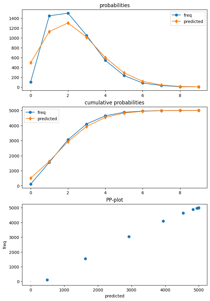
モデルを適合した後、poisson 診断クラスの plot 関数を使用して、期待予測分布と実現した頻度を比較できます。ポアソンモデルがゼロの数を過大評価し、1 と 2 の数を過小評価することを示しています。
[3]:
mod_p = Poisson(y, x)
res_p = mod_p.fit()
print(res_p.summary())
Optimization terminated successfully.
         Current function value: 1.668079
         Iterations 4
                          Poisson Regression Results
==============================================================================
Dep. Variable:                      y   No. Observations:                 5000
Model:                        Poisson   Df Residuals:                     4998
Method:                           MLE   Df Model:                            1
Date:                Thu, 03 Oct 2024   Pseudo R-squ.:                0.008678
Time:                        15:44:58   Log-Likelihood:                -8340.4
converged:                       True   LL-Null:                       -8413.4
Covariance Type:            nonrobust   LLR p-value:                 1.279e-33
==============================================================================
                 coef    std err          z      P>|z|      [0.025      0.975]
------------------------------------------------------------------------------
const          0.6532      0.019     33.642      0.000       0.615       0.691
x1             0.3871      0.032     12.062      0.000       0.324       0.450
==============================================================================
[4]:
dia_p = res_p.get_diagnostic()
dia_p.plot_probs();
ハードルモデルの推定
次に、正しく指定したポアソン-ポアソンハドルモデルを推定します。
HurdleCountModel の署名とオプションは、poisson-poisson が既定であることを示しているため、このモデルを作成するときはオプションを指定する必要はありません。
HurdleCountModel(endog, exog, offset=None, dist='poisson', zerodist='poisson', p=2, pzero=2, exposure=None, missing='none', **kwargs)
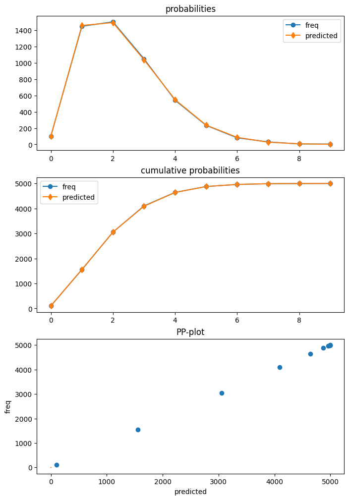
HurdleCountModel の results クラスには get_diagnostic メソッドがあります。ただし、診断メソッドの一部のみが現在利用可能です。予測分布のプロットは、データとの非常に高い一致を示しています。
[5]:
mod_h = HurdleCountModel(y, x)
res_h = mod_h.fit(disp=False)
print(res_h.summary())
                     HurdleCountModel Regression Results
==============================================================================
Dep. Variable:                      y   No. Observations:                 5000
Model:               HurdleCountModel   Df Residuals:                     4996
Method:                           MLE   Df Model:                            2
Date:                Thu, 03 Oct 2024   Pseudo R-squ.:                 0.01503
Time:                        15:44:59   Log-Likelihood:                -8004.9
converged:               [True, True]   LL-Null:                       -8127.1
Covariance Type:            nonrobust   LLR p-value:                 8.901e-54
==============================================================================
                 coef    std err          z      P>|z|      [0.025      0.975]
------------------------------------------------------------------------------
zm_const       0.9577      0.048     20.063      0.000       0.864       1.051
zm_x1          1.0576      0.121      8.737      0.000       0.820       1.295
const          0.5009      0.024     20.875      0.000       0.454       0.548
x1             0.4577      0.039     11.882      0.000       0.382       0.533
==============================================================================
[6]:
dia_h = res_h.get_diagnostic()
dia_h.plot_probs();
Wald 検定を使用して、ゼロモデルのパラメータがゼロ打ち切りカウントモデルのパラメータと同じかどうかをテストできます。p 値は非常に小さく、モデルが単なるポアソンであるという説を正しく否定しています。サンプルサイズが大きいので、この場合、検定の検出力が大きくなります。
[7]:
res_h.wald_test("zm_const = const, zm_x1 = x1", scalar=True)
[7]:
<class 'statsmodels.stats.contrast.ContrastResults'>
<Wald test (chi2): statistic=470.67320754391915, p-value=6.231772522807044e-103, df_denom=2>
予測
ハードルモデルは、全体のモデルと 2 つのサブモデルの統計量の予測に使用できます。予測するべき統計量は、which キーワードを使用して指定します。
以下は predict のドキュメント文字列から抜粋したもので、使用可能なオプションをリストしています。
which : str (optional)
    Statitistic to predict. Default is 'mean'.

    - 'mean' : the conditional expectation of endog E(y | x)
    - 'mean-main' : mean parameter of truncated count model.
      Note, this is not the mean of the truncated distribution.
    - 'linear' : the linear predictor of the truncated count model.
    - 'var' : returns the estimated variance of endog implied by the
      model.
    - 'prob-main' : probability of selecting the main model which is
      the probability of observing a nonzero count P(y > 0 | x).
    - 'prob-zero' : probability of observing a zero count. P(y=0 | x).
      This is equal to is ``1 - prob-main``
    - 'prob-trunc' : probability of truncation of the truncated count
      model. This is the probability of observing a zero count implied
      by the truncation model.
    - 'mean-nonzero' : expected value conditional on having observation
      larger than zero, E(y | X, y>0)
    - 'prob' : probabilities of each count from 0 to max(endog), or
      for y_values if those are provided. This is a multivariate
      return (2-dim when predicting for several observations).
これらのオプションは、results クラスの predict メソッドと get_prediction メソッドで使用できます。
次の例では、元のデータから等間隔で取得された説明変数のセットを作成します。その後、これらの説明変数で条件付けられた利用可能な統計量を予測できます。
[8]:
which_options = ["mean", "mean-main", "linear", "mean-nonzero", "prob-zero", "prob-main", "prob-trunc", "var", "prob"]
ex = x[slice(None, None, nobs // 5), :]
ex
[8]:
array([[1.        , 0.        ],
       [1.        , 0.20004001],
       [1.        , 0.40008002],
       [1.        , 0.60012002],
       [1.        , 0.80016003]])
[9]:
for w in which_options:
    print(w)
    pred = res_h.predict(ex, which=w)
    print("    ", pred)
mean
     [1.89150663 2.07648059 2.25555158 2.43319456 2.61673457]
mean-main
     [1.65015181 1.8083782  1.98177629 2.17180081 2.38004602]
linear
     [0.50086729 0.59243042 0.68399356 0.77555669 0.86711982]
mean-nonzero
     [2.04231955 2.16292424 2.29857565 2.45116551 2.62277411]
prob-zero
     [0.07384394 0.0399661  0.01871771 0.00733159 0.00230273]
prob-main
     [0.92615606 0.9600339  0.98128229 0.99266841 0.99769727]
prob-trunc
     [0.19202076 0.16391977 0.1378242  0.11397219 0.09254632]
var
     [1.43498239 1.51977118 1.63803729 1.7971727  1.99738345]
prob
     [[7.38439416e-02 3.63208532e-01 2.99674608e-01 1.64836199e-01
  6.80011882e-02 2.24424568e-02 6.17224344e-03 1.45501981e-03
  3.00125448e-04 5.50280612e-05]
 [3.99660987e-02 3.40376213e-01 3.07764462e-01 1.85518182e-01
  8.38717591e-02 3.03343722e-02 9.14266959e-03 2.36191491e-03
  5.33904431e-04 1.07277904e-04]
 [1.87177088e-02 3.10869602e-01 3.08037002e-01 2.03486809e-01
  1.00816333e-01 3.99590837e-02 1.31983274e-02 3.73659033e-03
  9.25635762e-04 2.03822556e-04]
 [7.33159258e-03 2.77316512e-01 3.01138113e-01 2.18003999e-01
  1.18365316e-01 5.14131777e-02 1.86098635e-02 5.77384524e-03
  1.56745522e-03 3.78244503e-04]
 [2.30272798e-03 2.42169151e-01 2.88186862e-01 2.28632665e-01
  1.36039066e-01 6.47558475e-02 2.56869828e-02 8.73374304e-03
  2.59833880e-03 6.87129546e-04]]
[10]:
for w in which_options[:-1]:
    print(w)
    pred = res_h.get_prediction(ex, which=w)
    print("    ", pred.predicted)
    print("  se", pred.se)
mean
     [1.89150663 2.07648059 2.25555158 2.43319456 2.61673457]
  se [0.07877461 0.05693768 0.05866892 0.09551274 0.15359057]
mean-main
     [1.65015181 1.8083782  1.98177629 2.17180081 2.38004602]
  se [0.03959242 0.03164634 0.02471869 0.02415162 0.03453261]
linear
     [0.50086729 0.59243042 0.68399356 0.77555669 0.86711982]
  se [0.04773779 0.03148549 0.02960421 0.04397859 0.06453261]
mean-nonzero
     [2.04231955 2.16292424 2.29857565 2.45116551 2.62277411]
  se [0.02978486 0.02443098 0.01958745 0.0196433  0.02881753]
prob-zero
     [0.07384394 0.0399661  0.01871771 0.00733159 0.00230273]
  se [0.00918583 0.00405155 0.00220446 0.00158494 0.00090255]
prob-main
     [0.92615606 0.9600339  0.98128229 0.99266841 0.99769727]
  se [0.00918583 0.00405155 0.00220446 0.00158494 0.00090255]
prob-trunc
     [0.19202076 0.16391977 0.1378242  0.11397219 0.09254632]
  se [0.00760257 0.00518746 0.00340683 0.00275261 0.00319587]
var
     [1.43498239 1.51977118 1.63803729 1.7971727  1.99738345]
  se [0.04853902 0.03615054 0.02747485 0.02655145 0.03733328]
/opt/hostedtoolcache/Python/3.10.15/x64/lib/python3.10/site-packages/statsmodels/base/_prediction_inference.py:782: UserWarning: using default log-link in get_prediction
  warnings.warn("using default log-link in get_prediction")
オプション which="prob" は、predict exog の各行の予測確率の配列を返します。多くの場合、すべての exog にわたって平均された平均確率に関心があります。予測メソッドには average=True オプションがあり、観測値の予測値の平均と、それらの平均予測の対応する標準誤差と信頼区間を計算できます。
[11]:
pred = res_h.get_prediction(ex, which="prob", average=True)
print("    ", pred.predicted)
print("  se", pred.se)
     [2.84324139e-02 3.06788002e-01 3.00960210e-01 2.00095571e-01
 1.01418732e-01 4.17809876e-02 1.45620174e-02 4.41222267e-03
 1.18509193e-03 2.86300514e-04]
  se [2.81472152e-03 5.00830805e-03 1.37524763e-03 1.87343644e-03
 1.99068649e-03 1.23878525e-03 5.78099173e-04 2.21180110e-04
 7.25021189e-05 2.08872558e-05]
panda DataFrame を使用して、より読みやすい表示を取得します。[予測済み] 列は、exog の 5 つのグリッドポイントの平均の応答値の予測分布の確率質量関数を示しています。確率は 1 に達しませんが、観測されたものよりも大きいカウントには正の確率があり、テーブルにはありません。ただし、この例ではその確率は小さくなります。
[12]:
dfp_h = pred.summary_frame()
dfp_h
[12]:
| 予測済み | se | ci_lower | ci_upper | |
|---|---|---|---|---|
| 0 | 0.028432 | 0.002815 | 0.022916 | 0.033949 |
| 1 | 0.306788 | 0.005008 | 0.296972 | 0.316604 |
| 2 | 0.300960 | 0.001375 | 0.298265 | 0.303656 |
| 3 | 0.200096 | 0.001873 | 0.196424 | 0.203767 |
| 4 | 0.101419 | 0.001991 | 0.097517 | 0.105320 |
| 5 | 0.041781 | 0.001239 | 0.039353 | 0.044209 |
| 6 | 0.014562 | 0.000578 | 0.013429 | 0.015695 |
| 7 | 0.004412 | 0.000221 | 0.003979 | 0.004846 |
| 8 | 0.001185 | 0.000073 | 0.001043 | 0.001327 |
| 9 | 0.000286 | 0.000021 | 0.000245 | 0.000327 |
[13]:
prob_larger9 = pred.predicted.sum()
prob_larger9, 1 - prob_larger9
[13]:
(np.float64(0.9999215487936677), np.float64(7.84512063323195e-05))
get_prediction は、この場合、基本 PredictionResultsDelta クラスのインスタンスを返します。
標準誤差、p 値、複数の分布パラメータに依存する非線形関数の信頼区間などの推測統計量は、デルタメソッドを使用して計算されます。予測の推論は、正規分布に基づいています。
[14]:
pred
[14]:
<statsmodels.base._prediction_inference.PredictionResultsDelta at 0x7f68ba217ee0>
[15]:
pred.dist, pred.dist_args
[15]:
(<scipy.stats._continuous_distns.norm_gen at 0x7f68c0dc2a40>, ())
ハードルモデルによって予測された分布を、以前に推定したポアソンモデルによって予測された分布と比較できます。最後の列「diff」は、ポアソンモデルは観測の約 8% だけゼロの数を過大評価し、1 と 2 のカウントを exog グリッドで平均してそれぞれ 7%、3.7%、過小評価していることを示しています。
[16]:
pred_p = res_p.get_prediction(ex, which="prob", average=True)
dfp_p = pred_p.summary_frame()
dfp_h["poisson"] = dfp_p["predicted"]
dfp_h["diff"] = dfp_h["poisson"] - dfp_h["predicted"]
dfp_h
[16]:
| 予測済み | se | ci_lower | ci_upper | ポアソン | diff | |
|---|---|---|---|---|---|---|
| 0 | 0.028432 | 0.002815 | 0.022916 | 0.033949 | 0.107848 | 0.079416 |
| 1 | 0.306788 | 0.005008 | 0.296972 | 0.316604 | 0.237020 | -0.069768 |
| 2 | 0.300960 | 0.001375 | 0.298265 | 0.303656 | 0.263523 | -0.037437 |
| 3 | 0.200096 | 0.001873 | 0.196424 | 0.203767 | 0.197657 | -0.002439 |
| 4 | 0.101419 | 0.001991 | 0.097517 | 0.105320 | 0.112511 | 0.011093 |
| 5 | 0.041781 | 0.001239 | 0.039353 | 0.044209 | 0.051833 | 0.010052 |
| 6 | 0.014562 | 0.000578 | 0.013429 | 0.015695 | 0.020124 | 0.005561 |
| 7 | 0.004412 | 0.000221 | 0.003979 | 0.004846 | 0.006769 | 0.002356 |
| 8 | 0.001185 | 0.000073 | 0.001043 | 0.001327 | 0.002012 | 0.000827 |
| 9 | 0.000286 | 0.000021 | 0.000245 | 0.000327 | 0.000537 | 0.000250 |
その他の推定後
推定されたハードルモデルは、パラメータのワルド検定と予測に使用できます。 対数尤度値や情報基準など、他の尤度最大統計量も使用できます。
ただし、推定、パラメータ推論、予測には不要で、ヘルパー関数を必要とする推定後のいくつかのメソッドは、まだ使用できません。 まだサポートされていない主なメソッドは、 score_test、 get_distribution、および get_influenceです。 get_diagnostics の診断対策は、予測に基づく統計にのみ使用できます。
[17]:
res_h.llf, res_h.df_resid, res_h.aic, res_h.bic
[17]:
(np.float64(-8004.904002793644),
 4996,
 np.float64(16017.808005587289),
 np.float64(16043.876778352953))
過剰分散はありますか? モデルが正しく指定されている場合は 1 に近づくべきピアソン残差を使用して、ピアソンカイ2統計量を計算できます。
[18]:
(res_h.resid_pearson**2).sum() / res_h.df_resid
[18]:
np.float64(0.9989670114949286)
診断クラスには、診断プロットで使用される予測分布もあります。 他の統計やテストは現在利用できません。
[19]:
dia_h.probs_predicted.mean(0)
[19]:
array([0.02044612, 0.29147174, 0.29856288, 0.20740118, 0.10990976,
       0.04737579, 0.0172898 , 0.00548983, 0.00154646, 0.00039214])
[20]:
res_h.resid[:10]
[20]:
array([ 1.10849337,  1.10830496, -0.89188344, -0.89207183,  1.10773978,
       -0.8924486 , -0.89263697,  0.10717466,  0.1069863 ,  0.10679794])
[ ]: