推定後概要 - ポアソン
このノートブックは、ポアソンモデルを例として、いくつかのモデルで使用可能な推定後の結果の概要を示しています。
参照: https://github.com/statsmodels/statsmodels/issues/7707
従来、モデルのresultsクラスはワルド推論と予測を提供していました。現在、多くのモデルは、推定後の結果、推論、予測、および仕様または診断テストのための追加メソッドを備えています。
以下は、主に離散モデルについて、tsa以外の最尤モデルの現在のパターンに基づいています。他のモデルでは、ある程度異なるAPIパターンに従っています。OLSやWLSなどの線形モデルは、独自の特別な実装(例えばOLSの影響)を持っています。GLMにも、モデル固有の機能がいくつか残っています。
主な推定後機能は次のとおりです。
推論 - ワルド検定 セクション
推論 - スコア検定 セクション
get_prediction推論統計を含む予測 セクションget_distribution推定パラメータに基づく分布クラス セクションget_diagnostic診断と仕様テスト、尺度、プロット セクションget_influence外れ値と影響の診断 セクション
シミュレーションされた例
説明のために、正しく指定され、比較的大きなサンプルを持つポアソン回帰のデータをシミュレートします。1つの回帰変数は2レベルのカテゴリ変数です。2番目の回帰変数は単位区間で一様に分布しています。
[1]:
import numpy as np
import pandas as pd
from scipy import stats
import matplotlib.pyplot as plt

from statsmodels.discrete.discrete_model import Poisson
from statsmodels.discrete.diagnostic import PoissonDiagnostic
[2]:
np.random.seed(983154356)

nr = 10
n_groups = 2
labels = np.arange(n_groups)
x = np.repeat(labels, np.array([40, 60]) * nr)
nobs = x.shape[0]
exog = (x[:, None] == labels).astype(np.float64)
xc = np.random.rand(len(x))
exog = np.column_stack((exog, xc))
# reparameterize to explicit constant
# exog[:, 1] = 1
beta = np.array([0.2, 0.3, 0.5], np.float64)

linpred = exog @ beta
mean = np.exp(linpred)
y = np.random.poisson(mean)
len(y), y.mean(), (y == 0).mean()

res = Poisson(y, exog).fit(disp=0)
print(res.summary())
                          Poisson Regression Results
==============================================================================
Dep. Variable:                      y   No. Observations:                 1000
Model:                        Poisson   Df Residuals:                      997
Method:                           MLE   Df Model:                            2
Date:                Thu, 03 Oct 2024   Pseudo R-squ.:                 0.01258
Time:                        15:46:52   Log-Likelihood:                -1618.3
converged:                       True   LL-Null:                       -1638.9
Covariance Type:            nonrobust   LLR p-value:                 1.120e-09
==============================================================================
                 coef    std err          z      P>|z|      [0.025      0.975]
------------------------------------------------------------------------------
x1             0.2386      0.061      3.926      0.000       0.120       0.358
x2             0.3229      0.055      5.873      0.000       0.215       0.431
x3             0.5109      0.083      6.186      0.000       0.349       0.673
==============================================================================
[ ]:
推論 - ワルド検定
fitのcov_typeオプション)。パラメーターテーブルの統計以外に、現在使用可能なメソッドは次のとおりです。
t_test
wald_test
t_test_pairwise
wald_test_terms
f_testはレガシーメソッドとして使用できます。use_f=Trueキーワードオプションを使用したwald_testと同じです。
[3]:
res.t_test("x1=x2")
[3]:
<class 'statsmodels.stats.contrast.ContrastResults'>
                             Test for Constraints
==============================================================================
                 coef    std err          z      P>|z|      [0.025      0.975]
------------------------------------------------------------------------------
c0            -0.0843      0.049     -1.717      0.086      -0.181       0.012
==============================================================================
[4]:
res.wald_test("x1=x2, x3", scalar=True)
[4]:
<class 'statsmodels.stats.contrast.ContrastResults'>
<Wald test (chi2): statistic=40.772322944293464, p-value=1.4008852592190214e-09, df_denom=2>
推論 - スコア検定
statsmodels 0.14で、ほとんどの離散モデルとGLMに追加されました。
スコア検定またはラグランジュ乗数(LM)検定は、帰無仮説の下で推定されたモデルに基づいています。一般的な例として、追加変数の統計的有意性を検定するために、帰無制約の下でモデルパラメーターを推定しますが、追加変数の統計的有意性を検定するために、完全モデルの下でスコアとヘッセ行列を評価する変数追加検定があります。
仕様検定に、変数追加スコア検定を使用できます。次の例では、2次項または多項式項を追加することで、モデルに誤指定された非線形性があるかどうかを検定します。
この例では、モデルは正しく指定されており、サンプルサイズが大きいため、これらの仕様検定では帰無仮説が棄却されないことが予想されます。
[5]:
res.score_test(exog_extra=xc**2)
[5]:
(array([0.05300569]), array([0.81791332]), 1)
[6]:
linpred = res.predict(which="linear")
res.score_test(exog_extra=linpred[:,None]**[2, 3])
[6]:
(array([1.3867703]), array([0.49988103]), 2)
予測
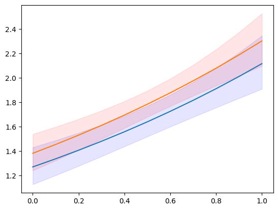
モデルとresultsクラスには、予測値のみを返すpredictメソッドがあります。get_predictionメソッドは、予測、標準誤差、p値、信頼区間に対する推論統計を追加します。
次の例では、カテゴリレベルで分割され、連続変数の均一なグリッド上に配置された、新しい説明変数のセットを作成します。
[7]:
n = 11
exc = np.linspace(0, 1, n)
ex1 = np.column_stack((np.ones(n), np.zeros(n), exc))
ex2 = np.column_stack((np.zeros(n), np.ones(n), exc))

m1 = res.get_prediction(ex1)
m2 = res.get_prediction(ex2)
予測結果クラスで使用可能なメソッドと属性は次のとおりです。
[8]:
[i for i in dir(m1) if not i.startswith("_")]
[8]:
['conf_int',
 'deriv',
 'df',
 'dist',
 'dist_args',
 'func',
 'linpred',
 'linpred_se',
 'predicted',
 'row_labels',
 'se',
 'summary_frame',
 't_test',
 'tvalues',
 'var_pred']
[9]:
plt.plot(exc, np.column_stack([m1.predicted, m2.predicted]))
ci = m1.conf_int()
plt.fill_between(exc, ci[:, 0], ci[:, 1], color='b', alpha=.1)
ci = m2.conf_int()
plt.fill_between(exc, ci[:, 0], ci[:, 1], color='r', alpha=.1)
# to add observed points:
# y1 = y[x == 0]
# plt.plot(xc[x == 0], y1, ".", color="b", alpha=.3)
# y2 = y[x == 1]
# plt.plot(xc[x == 1], y2, ".", color="r", alpha=.3)
[9]:
<matplotlib.collections.PolyCollection at 0x7f852a5340a0>
[10]:
y.max()
[10]:
np.int64(7)
予測可能な統計の1つ(「which」キーワードで指定)は、予測分布の期待頻度または確率です。これにより、特定の説明変数のセットに対して、カウント=1、2、3、…を観察する予測確率がわかります。
[11]:
y_max = 5
f1 = res.get_prediction(ex1, which="prob", y_values=np.arange(y_max + 1))
f2 = res.get_prediction(ex2, which="prob", y_values=np.arange(y_max + 1))
f1.predicted.mean(0), f2.predicted.mean(0)
[11]:
(array([0.19681697, 0.31325239, 0.25570764, 0.14275759, 0.06128168,
        0.02154715]),
 array([0.17115113, 0.29529781, 0.26128059, 0.15810937, 0.07357482,
        0.02804883]))
予測確率の信頼区間を取得することもできます。ただし、平均予測確率の信頼区間が必要な場合は、predict関数内で集計する必要があります。関連するキーワードは「average」であり、exog配列で指定された観測値全体での予測の平均を計算します。
[12]:
f1 = res.get_prediction(ex1, which="prob", y_values=np.arange(y_max + 1), average=True)
f2 = res.get_prediction(ex2, which="prob", y_values=np.arange(y_max + 1), average=True)
f1.predicted, f2.predicted
[12]:
(array([0.19681697, 0.31325239, 0.25570764, 0.14275759, 0.06128168,
        0.02154715]),
 array([0.17115113, 0.29529781, 0.26128059, 0.15810937, 0.07357482,
        0.02804883]))
[13]:
f1.conf_int()
[13]:
array([[0.17256941, 0.22106453],
       [0.2982307 , 0.32827408],
       [0.24818616, 0.26322912],
       [0.12876732, 0.15674787],
       [0.05088296, 0.07168041],
       [0.01626921, 0.0268251 ]])
[14]:
f2.conf_int()
[14]:
array([[0.15303084, 0.18927142],
       [0.28178041, 0.30881522],
       [0.25622062, 0.26634055],
       [0.14720224, 0.1690165 ],
       [0.06442055, 0.0827291 ],
       [0.02287077, 0.03322688]])
help(res.get_prediction)help(res.model.predict)分布
特定のパラメーターに対して、scipyまたはscipy互換の分布クラスのインスタンスを作成できます。これにより、分布のメソッド(pmf/pdf、cdf、statsなど)にアクセスできます。
resultsクラスのget_distributionメソッドは、提供された説明変数の配列と推定パラメーターを使用して、ベクトル化された分布を指定します。モデルのget_predictionメソッドは、ユーザー指定のパラメーターparamsに使用できます。
[15]:
distr = res.get_distribution()
distr
[15]:
<scipy.stats._distn_infrastructure.rv_discrete_frozen at 0x7f852a592e30>
[16]:
distr.pmf(0)[:10]
[16]:
array([0.15420516, 0.13109359, 0.17645042, 0.16735421, 0.13445031,
       0.14851843, 0.22287053, 0.14979318, 0.25252986, 0.25013583])
条件付き分布の平均は、モデルからの予測平均と同じです。
[17]:
distr.mean()[:10]
[17]:
array([1.86947133, 2.03184379, 1.73471534, 1.78764267, 2.00656061,
       1.90704623, 1.50116427, 1.89849971, 1.37622577, 1.3857512 ])
[18]:
res.predict()[:10]
[18]:
array([1.86947133, 2.03184379, 1.73471534, 1.78764267, 2.00656061,
       1.90704623, 1.50116427, 1.89849971, 1.37622577, 1.3857512 ])
新しい説明変数のセットについても分布を取得できます。説明変数は、predictメソッドと同様の方法で提供できます。
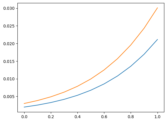
予測セクションの説明変数のグリッドを再利用します。使用方法の例として、説明変数の値を条件として、5より大きい(厳密に)カウントを観察する確率を計算できます。
[19]:
distr1 = res.get_distribution(ex1)
distr2 = res.get_distribution(ex2)
[20]:
distr1.sf(5), distr2.sf(5)
[20]:
(array([0.00198421, 0.00255027, 0.00326858, 0.00417683, 0.00532093,
        0.00675641, 0.00854998, 0.01078116, 0.0135439 , 0.01694825,
        0.02112179]),
 array([0.00299758, 0.00383456, 0.00489029, 0.00621677, 0.00787663,
        0.00994468, 0.01250966, 0.01567579, 0.01956437, 0.02431503,
        0.03008666]))
[21]:
plt.plot(exc, np.column_stack([distr1.sf(5), distr2.sf(5)]))
[21]:
[<matplotlib.lines.Line2D at 0x7f852a42cb50>,
 <matplotlib.lines.Line2D at 0x7f852a42cc40>]
分布を使用して、新しい観測値の上側信頼限界を見つけることもできます。次のプロットとテーブルは、特定の説明変数に対する上限カウントを示しています。このカウント以下の値を観察する確率は少なくとも0.99です。
これは、パラメーターを固定値として扱い、パラメーターの不確実性を考慮していないことに注意してください。
[22]:
plt.plot(exc, np.column_stack([distr1.ppf(0.99), distr2.ppf(0.99)]))
[22]:
[<matplotlib.lines.Line2D at 0x7f852a536140>,
 <matplotlib.lines.Line2D at 0x7f852a5358a0>]
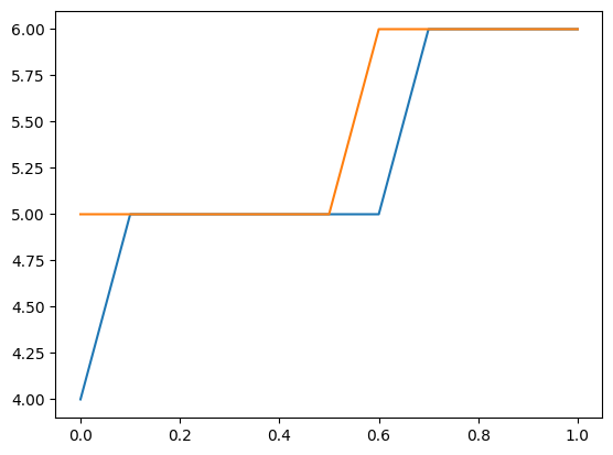
[23]:
[distr1.ppf(0.99), distr2.ppf(0.99)]
[23]:
[array([4., 5., 5., 5., 5., 5., 5., 6., 6., 6., 6.]),
 array([5., 5., 5., 5., 5., 5., 6., 6., 6., 6., 6.])]
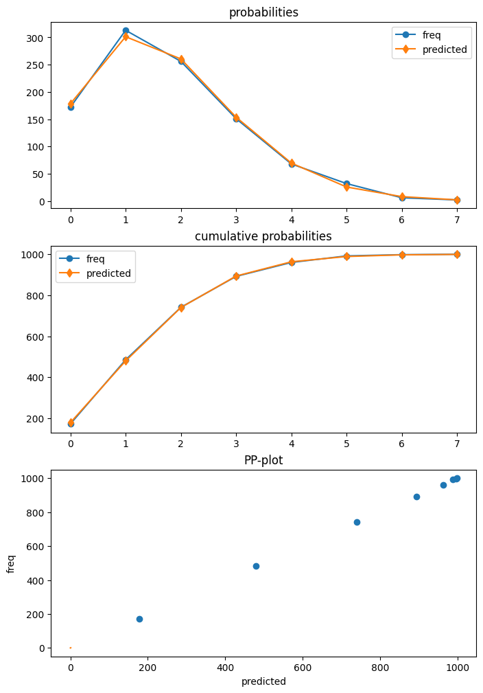
診断
ポアソンは、get_diagnosticを使用して結果から取得できる診断クラスを持つ最初のモデルです。他のカウントモデルは、現在メソッド数が限られている一般的なカウント診断クラスを持っています。
この例でのポアソンモデルは正しく指定されています。さらに、サンプルサイズが大きいです。そのため、このケースでは、診断テストのいずれも、正しい仕様の帰無仮説を棄却しません。
[24]:
dia = res.get_diagnostic()
[i for i in dir(dia) if not i.startswith("_")]
[24]:
['plot_probs',
 'probs_predicted',
 'results',
 'test_chisquare_prob',
 'test_dispersion',
 'test_poisson_zeroinflation',
 'y_max']
[25]:
dia.plot_probs();
過剰分散の検定
ポアソンにはいくつかの分散検定があります。現在、それらはすべて返されます。DispersionResultsクラスには、summary_frameメソッドがあります。返されるデータフレームは、読みやすい結果の概要を提供します。
[26]:
td = dia.test_dispersion()
td
[26]:
<class 'statsmodels.discrete._diagnostics_count.DispersionResults'>
statistic = array([-0.42597379, -0.42597379, -0.39884024, -0.48327447, -0.48327447,
           -0.47790855, -0.45225818])
pvalue = array([0.67012695, 0.67012695, 0.69001092, 0.62890087, 0.62890087,
           0.6327153 , 0.651083  ])
method = ['Dean A', 'Dean B', 'Dean C', 'CT nb2', 'CT nb1', 'CT nb2 HC3', 'CT nb1 HC3']
alternative = ['mu (1 + a mu)', 'mu (1 + a mu)', 'mu (1 + a)', 'mu (1 + a mu)', 'mu (1 + a)', 'mu (1 + a mu)', 'mu (1 + a)']
name = 'Poisson Dispersion Test'
tuple = (array([-0.42597379, -0.42597379, -0.39884024, -0.48327447, -0.48327447,
           -0.47790855, -0.45225818]), array([0.67012695, 0.67012695, 0.69001092, 0.62890087, 0.62890087,
           0.6327153 , 0.651083  ]))
[27]:
df = td.summary_frame()
df
[27]:
| 統計量 | p値 | 方法 | 対立仮説 | |
|---|---|---|---|---|
| 0 | -0.425974 | 0.670127 | ディーンA | μ(1 + aμ) |
| 1 | -0.425974 | 0.670127 | ディーンB | μ(1 + aμ) |
| 2 | -0.398840 | 0.690011 | ディーンC | μ(1 + a) |
| 3 | -0.483274 | 0.628901 | CT nb2 | μ(1 + aμ) |
| 4 | -0.483274 | 0.628901 | CT nb1 | μ(1 + a) |
| 5 | -0.477909 | 0.632715 | CT nb2 HC3 | μ(1 + aμ) |
| 6 | -0.452258 | 0.651083 | CT nb1 HC3 | μ(1 + a) |
ゼロインフレの検定
[28]:
dia.test_poisson_zeroinflation()
[28]:
<class 'statsmodels.stats.base.HolderTuple'>
statistic = np.float64(-0.6657556201098714)
pvalue = np.float64(0.5055673158225651)
pvalue_smaller = np.float64(0.7472163420887175)
pvalue_larger = np.float64(0.25278365791128254)
chi2 = np.float64(0.44323054570787945)
pvalue_chi2 = np.float64(0.505567315822565)
df_chi2 = 1
distribution = 'normal'
tuple = (np.float64(-0.6657556201098714), np.float64(0.5055673158225651))
ゼロインフレに対するカイ二乗検定
[29]:
dia.test_chisquare_prob(bin_edges=np.arange(3))
[29]:
<class 'statsmodels.stats.base.HolderTuple'>
statistic = np.float64(0.456170941873113)
pvalue = np.float64(0.4994189468121014)
df = np.int64(1)
diff1 = array([[-0.15420516,  0.71171787],
           [-0.13109359, -0.26636169],
           [-0.17645042, -0.30609125],
           ...,
           [-0.10477112, -0.23636125],
           [-0.10675436, -0.2388335 ],
           [-0.21168332, -0.32867305]])
res_aux = <statsmodels.regression.linear_model.RegressionResultsWrapper object at 0x7f852a290eb0>
distribution = 'chi2'
tuple = (np.float64(0.456170941873113), np.float64(0.4994189468121014))
予測頻度に対する適合度検定
これは、パラメータが推定されていることを考慮したカイ二乗検定です。最大ビンエッジより大きいカウントは最後のビンに追加されるため、ビンの合計は1になります。
例として、5つのビンを使用する場合
[30]:
dt = dia.test_chisquare_prob(bin_edges=np.arange(6))
dt
[30]:
<class 'statsmodels.stats.base.HolderTuple'>
statistic = np.float64(0.9414641297779136)
pvalue = np.float64(0.9185382008345917)
df = np.int64(4)
diff1 = array([[-0.15420516,  0.71171787, -0.26946759, -0.16792064, -0.07848071],
           [-0.13109359, -0.26636169, -0.27060268,  0.81672588, -0.0930961 ],
           [-0.17645042, -0.30609125,  0.7345094 , -0.15351687, -0.06657702],
           ...,
           [-0.10477112, -0.23636125, -0.26661279,  0.79950922, -0.11307565],
           [-0.10675436, -0.2388335 ,  0.73283789, -0.1992339 , -0.11143275],
           [-0.21168332, -0.32867305,  0.74484061, -0.13205892, -0.05126078]])
res_aux = <statsmodels.regression.linear_model.RegressionResultsWrapper object at 0x7f852a27a7d0>
distribution = 'chi2'
tuple = (np.float64(0.9414641297779136), np.float64(0.9185382008345917))
[31]:
dt.diff1.mean(0)
[31]:
array([-0.00628136, 0.01177308, -0.00449604, -0.00270524, -0.00156519])
[32]:
vars(dia)
[32]:
{'results': <statsmodels.discrete.discrete_model.PoissonResults at 0x7f85761bdcf0>,
 'y_max': None,
 '_cache': {'probs_predicted': array([[0.15420516, 0.28828213, 0.26946759, ..., 0.02934349, 0.0091428 ,
          0.00244174],
         [0.13109359, 0.26636169, 0.27060268, ..., 0.03783135, 0.01281123,
          0.00371863],
         [0.17645042, 0.30609125, 0.2654906 , ..., 0.02309843, 0.0066782 ,
          0.00165497],
         ...,
         [0.10477112, 0.23636125, 0.26661279, ..., 0.05101921, 0.01918303,
          0.00618235],
         [0.10675436, 0.2388335 , 0.26716211, ..., 0.04986002, 0.01859135,
          0.00594186],
         [0.21168332, 0.32867305, 0.25515939, ..., 0.01591815, 0.00411926,
          0.00091369]])}}
外れ値と影響力
Statsmodelsは、非線形モデル(非線形期待平均を持つモデル)に対して一般的なMLEInfluenceクラスを提供します。これは、離散モデルやベータ回帰モデルなどの他の最尤推定に基づくモデルにも適用されます。提供される尺度は一般的な定義に基づいており、例えば線形モデルにおけるハット行列の対角要素ではなく、一般化されたてこ比を使用しています。
resultsメソッドget_influenceは、外れ値と影響力の尺度に関する様々なメソッドを持つMLEInfluenceクラスのインスタンスを返します。
[33]:
infl = res.get_influence()
[i for i in dir(infl) if not i.startswith("_")]
[33]:
['cooks_distance',
 'cov_params',
 'd_fittedvalues',
 'd_fittedvalues_scaled',
 'd_params',
 'dfbetas',
 'endog',
 'exog',
 'hat_matrix_diag',
 'hat_matrix_exog_diag',
 'hessian',
 'k_params',
 'k_vars',
 'model_class',
 'nobs',
 'params_one',
 'plot_index',
 'plot_influence',
 'resid',
 'resid_score',
 'resid_score_factor',
 'resid_studentized',
 'results',
 'scale',
 'score_obs',
 'summary_frame']
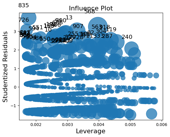
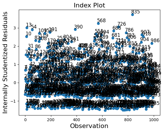
influenceクラスには2つのプロットメソッドがあります。しかし、サンプルサイズが大きいため、この場合、プロットは非常に混雑しています。
[34]:
infl.plot_influence();
[35]:
infl.plot_index(y_var="resid_studentized");
summary_frameは、各観測値の主要な影響と外れ値の尺度を示します。
私たちの例では1000個の観測値があり、これは表示するには多すぎます。要約データフレームを列のいずれかでソートし、最も大きい外れ値または影響力の尺度を持つ観測値をリストすることができます。以下の例では、クックの距離とstandard_resid(一般的なケースではピアソンの残差)でソートします。
「良好な」モデルをシミュレートしたため、大きな影響力を持つ観測値や大きな外れ値はありません。
[36]:
df_infl = infl.summary_frame()
df_infl.head()
[36]:
| dfb_x1 | dfb_x2 | dfb_x3 | クックの距離 | 標準化残差 | ハット行列の対角要素 | dffits_internal | |
|---|---|---|---|---|---|---|---|
| 0 | -0.010856 | 0.011384 | -0.013643 | 0.000440 | -0.636944 | 0.003243 | -0.036334 |
| 1 | 0.001990 | -0.023625 | 0.028313 | 0.000737 | 0.680823 | 0.004749 | 0.047031 |
| 2 | 0.005794 | -0.000787 | 0.000943 | 0.000035 | 0.201681 | 0.002607 | 0.010311 |
| 3 | -0.014243 | 0.005539 | -0.006639 | 0.000325 | -0.589923 | 0.002790 | -0.031206 |
| 4 | 0.003602 | -0.022549 | 0.027024 | 0.000738 | 0.702888 | 0.004462 | 0.047057 |
[37]:
df_infl.sort_values("cooks_d", ascending=False)[:10]
[37]:
| dfb_x1 | dfb_x2 | dfb_x3 | クックの距離 | 標準化残差 | ハット行列の対角要素 | dffits_internal | |
|---|---|---|---|---|---|---|---|
| 568 | -0.110520 | -0.038997 | 0.143106 | 0.013922 | 3.236167 | 0.003972 | 0.204365 |
| 13 | 0.048914 | -0.056713 | 0.067969 | 0.010034 | 3.011778 | 0.003307 | 0.173497 |
| 918 | -0.093971 | -0.038431 | 0.121677 | 0.009304 | 2.519367 | 0.004378 | 0.167066 |
| 563 | -0.089917 | -0.033708 | 0.116428 | 0.008935 | 2.545624 | 0.004119 | 0.163720 |
| 119 | 0.163230 | 0.103957 | -0.124589 | 0.008883 | 2.409646 | 0.004569 | 0.163247 |
| 390 | 0.148697 | 0.066972 | -0.080264 | 0.008358 | 2.907190 | 0.002958 | 0.158345 |
| 835 | -0.017672 | 0.066475 | 0.022883 | 0.008209 | 3.727645 | 0.001769 | 0.156931 |
| 54 | 0.145944 | 0.064216 | -0.076961 | 0.008156 | 2.892554 | 0.002916 | 0.156419 |
| 907 | -0.078901 | -0.020908 | 0.102164 | 0.008021 | 2.615676 | 0.003505 | 0.155126 |
| 304 | 0.152905 | 0.093680 | -0.112272 | 0.007821 | 2.351520 | 0.004225 | 0.153179 |
[38]:
df_infl.sort_values("standard_resid", ascending=False)[:10]
[38]:
| dfb_x1 | dfb_x2 | dfb_x3 | クックの距離 | 標準化残差 | ハット行列の対角要素 | dffits_internal | |
|---|---|---|---|---|---|---|---|
| 835 | -0.017672 | 0.066475 | 0.022883 | 0.008209 | 3.727645 | 0.001769 | 0.156931 |
| 568 | -0.110520 | -0.038997 | 0.143106 | 0.013922 | 3.236167 | 0.003972 | 0.204365 |
| 726 | -0.003941 | 0.065200 | 0.005103 | 0.005303 | 3.056406 | 0.001700 | 0.126127 |
| 13 | 0.048914 | -0.056713 | 0.067969 | 0.010034 | 3.011778 | 0.003307 | 0.173497 |
| 390 | 0.148697 | 0.066972 | -0.080264 | 0.008358 | 2.907190 | 0.002958 | 0.158345 |
| 54 | 0.145944 | 0.064216 | -0.076961 | 0.008156 | 2.892554 | 0.002916 | 0.156419 |
| 688 | 0.083205 | 0.148254 | -0.107737 | 0.007606 | 2.833988 | 0.002833 | 0.151057 |
| 191 | 0.122062 | 0.040388 | -0.048403 | 0.006704 | 2.764369 | 0.002625 | 0.141815 |
| 786 | -0.061179 | -0.000408 | 0.079217 | 0.006827 | 2.724900 | 0.002751 | 0.143110 |
| 109 | 0.110999 | 0.029401 | -0.035236 | 0.006212 | 2.704144 | 0.002542 | 0.136518 |