一般化線形モデル
[1]:
%matplotlib inline
[2]:
import numpy as np
import statsmodels.api as sm
from scipy import stats
from matplotlib import pyplot as plt

plt.rc("figure", figsize=(16,8))
plt.rc("font", size=14)
GLM: 二項応答データ
Star98 データの読み込み
この例では、Jeff Gill (2000) Generalized linear models: A unified approach から許可を得て取得した Star98 データセットを使用します。コードブック情報は、次のように入力することで取得できます。
[3]:
print(sm.datasets.star98.NOTE)
::

    Number of Observations - 303 (counties in California).

    Number of Variables - 13 and 8 interaction terms.

    Definition of variables names::

        NABOVE   - Total number of students above the national median for the
                   math section.
        NBELOW   - Total number of students below the national median for the
                   math section.
        LOWINC   - Percentage of low income students
        PERASIAN - Percentage of Asian student
        PERBLACK - Percentage of black students
        PERHISP  - Percentage of Hispanic students
        PERMINTE - Percentage of minority teachers
        AVYRSEXP - Sum of teachers' years in educational service divided by the
                number of teachers.
        AVSALK   - Total salary budget including benefits divided by the number
                   of full-time teachers (in thousands)
        PERSPENK - Per-pupil spending (in thousands)
        PTRATIO  - Pupil-teacher ratio.
        PCTAF    - Percentage of students taking UC/CSU prep courses
        PCTCHRT  - Percentage of charter schools
        PCTYRRND - Percentage of year-round schools

        The below variables are interaction terms of the variables defined
        above.

        PERMINTE_AVYRSEXP
        PEMINTE_AVSAL
        AVYRSEXP_AVSAL
        PERSPEN_PTRATIO
        PERSPEN_PCTAF
        PTRATIO_PCTAF
        PERMINTE_AVTRSEXP_AVSAL
        PERSPEN_PTRATIO_PCTAF
データを読み込み、定数を外生(独立)変数に追加します
[4]:
data = sm.datasets.star98.load()
data.exog = sm.add_constant(data.exog, prepend=False)
従属変数は N x 2 です(成功:NABOVE、失敗:NBELOW)
[5]:
print(data.endog.head())
   NABOVE  NBELOW
0   452.0   355.0
1   144.0    40.0
2   337.0   234.0
3   395.0   178.0
4     8.0    57.0
独立変数には、上記で説明した他のすべての変数と、交互作用項が含まれます
[6]:
print(data.exog.head())
     LOWINC   PERASIAN   PERBLACK    PERHISP  PERMINTE  AVYRSEXP    AVSALK  \
0  34.39730  23.299300  14.235280  11.411120  15.91837  14.70646  59.15732
1  17.36507  29.328380   8.234897   9.314884  13.63636  16.08324  59.50397
2  32.64324   9.226386  42.406310  13.543720  28.83436  14.59559  60.56992
3  11.90953  13.883090   3.796973  11.443110  11.11111  14.38939  58.33411
4  36.88889  12.187500  76.875000   7.604167  43.58974  13.90568  63.15364

   PERSPENK   PTRATIO     PCTAF  ...   PCTYRRND  PERMINTE_AVYRSEXP  \
0  4.445207  21.71025  57.03276  ...  22.222220         234.102872
1  5.267598  20.44278  64.62264  ...   0.000000         219.316851
2  5.482922  18.95419  53.94191  ...   0.000000         420.854496
3  4.165093  21.63539  49.06103  ...   7.142857         159.882095
4  4.324902  18.77984  52.38095  ...   0.000000         606.144976

   PERMINTE_AVSAL  AVYRSEXP_AVSAL  PERSPEN_PTRATIO  PERSPEN_PCTAF  \
0       941.68811        869.9948         96.50656      253.52242
1       811.41756        957.0166        107.68435      340.40609
2      1746.49488        884.0537        103.92435      295.75929
3       648.15671        839.3923         90.11341      204.34375
4      2752.85075        878.1943         81.22097      226.54248

   PTRATIO_PCTAF  PERMINTE_AVYRSEXP_AVSAL  PERSPEN_PTRATIO_PCTAF  const
0      1238.1955               13848.8985              5504.0352    1.0
1      1321.0664               13050.2233              6958.8468    1.0
2      1022.4252               25491.1232              5605.8777    1.0
3      1061.4545                9326.5797              4421.0568    1.0
4       983.7059               38280.2616              4254.4314    1.0

[5 rows x 21 columns]
適合とサマリー
[7]:
glm_binom = sm.GLM(data.endog, data.exog, family=sm.families.Binomial())
res = glm_binom.fit()
print(res.summary())
                  Generalized Linear Model Regression Results
================================================================================
Dep. Variable:     ['NABOVE', 'NBELOW']   No. Observations:                  303
Model:                              GLM   Df Residuals:                      282
Model Family:                  Binomial   Df Model:                           20
Link Function:                    Logit   Scale:                          1.0000
Method:                            IRLS   Log-Likelihood:                -2998.6
Date:                  Thu, 03 Oct 2024   Deviance:                       4078.8
Time:                          15:46:26   Pearson chi2:                 4.05e+03
No. Iterations:                       5   Pseudo R-squ. (CS):              1.000
Covariance Type:              nonrobust
===========================================================================================
                              coef    std err          z      P>|z|      [0.025      0.975]
-------------------------------------------------------------------------------------------
LOWINC                     -0.0168      0.000    -38.749      0.000      -0.018      -0.016
PERASIAN                    0.0099      0.001     16.505      0.000       0.009       0.011
PERBLACK                   -0.0187      0.001    -25.182      0.000      -0.020      -0.017
PERHISP                    -0.0142      0.000    -32.818      0.000      -0.015      -0.013
PERMINTE                    0.2545      0.030      8.498      0.000       0.196       0.313
AVYRSEXP                    0.2407      0.057      4.212      0.000       0.129       0.353
AVSALK                      0.0804      0.014      5.775      0.000       0.053       0.108
PERSPENK                   -1.9522      0.317     -6.162      0.000      -2.573      -1.331
PTRATIO                    -0.3341      0.061     -5.453      0.000      -0.454      -0.214
PCTAF                      -0.1690      0.033     -5.169      0.000      -0.233      -0.105
PCTCHRT                     0.0049      0.001      3.921      0.000       0.002       0.007
PCTYRRND                   -0.0036      0.000    -15.878      0.000      -0.004      -0.003
PERMINTE_AVYRSEXP          -0.0141      0.002     -7.391      0.000      -0.018      -0.010
PERMINTE_AVSAL             -0.0040      0.000     -8.450      0.000      -0.005      -0.003
AVYRSEXP_AVSAL             -0.0039      0.001     -4.059      0.000      -0.006      -0.002
PERSPEN_PTRATIO             0.0917      0.015      6.321      0.000       0.063       0.120
PERSPEN_PCTAF               0.0490      0.007      6.574      0.000       0.034       0.064
PTRATIO_PCTAF               0.0080      0.001      5.362      0.000       0.005       0.011
PERMINTE_AVYRSEXP_AVSAL     0.0002   2.99e-05      7.428      0.000       0.000       0.000
PERSPEN_PTRATIO_PCTAF      -0.0022      0.000     -6.445      0.000      -0.003      -0.002
const                       2.9589      1.547      1.913      0.056      -0.073       5.990
===========================================================================================
関心のある量
[8]:
print('Total number of trials:',  data.endog.iloc[:, 0].sum())
print('Parameters: ', res.params)
print('T-values: ', res.tvalues)
Total number of trials: 108418.0
Parameters:  LOWINC                    -0.016815
PERASIAN                   0.009925
PERBLACK                  -0.018724
PERHISP                   -0.014239
PERMINTE                   0.254487
AVYRSEXP                   0.240694
AVSALK                     0.080409
PERSPENK                  -1.952161
PTRATIO                   -0.334086
PCTAF                     -0.169022
PCTCHRT                    0.004917
PCTYRRND                  -0.003580
PERMINTE_AVYRSEXP         -0.014077
PERMINTE_AVSAL            -0.004005
AVYRSEXP_AVSAL            -0.003906
PERSPEN_PTRATIO            0.091714
PERSPEN_PCTAF              0.048990
PTRATIO_PCTAF              0.008041
PERMINTE_AVYRSEXP_AVSAL    0.000222
PERSPEN_PTRATIO_PCTAF     -0.002249
const                      2.958878
dtype: float64
T-values:  LOWINC                    -38.749083
PERASIAN                   16.504736
PERBLACK                  -25.182189
PERHISP                   -32.817913
PERMINTE                    8.498271
AVYRSEXP                    4.212479
AVSALK                      5.774998
PERSPENK                   -6.161911
PTRATIO                    -5.453217
PCTAF                      -5.168654
PCTCHRT                     3.921200
PCTYRRND                  -15.878260
PERMINTE_AVYRSEXP          -7.390931
PERMINTE_AVSAL             -8.449639
AVYRSEXP_AVSAL             -4.059162
PERSPEN_PTRATIO             6.321099
PERSPEN_PCTAF               6.574347
PTRATIO_PCTAF               5.362290
PERMINTE_AVYRSEXP_AVSAL     7.428064
PERSPEN_PTRATIO_PCTAF      -6.445137
const                       1.913012
dtype: float64
最初の差分:すべての説明変数を平均値に固定し、低所得世帯の割合を操作して、応答変数への影響を評価します
[9]:
means = data.exog.mean(axis=0)
means25 = means.copy()
means25.iloc[0] = stats.scoreatpercentile(data.exog.iloc[:,0], 25)
means75 = means.copy()
means75.iloc[0] = lowinc_75per = stats.scoreatpercentile(data.exog.iloc[:,0], 75)
resp_25 = res.predict(means25)
resp_75 = res.predict(means75)
diff = resp_75 - resp_25
学区における低所得世帯の割合の四分位範囲の最初の差分は次のとおりです。
[10]:
print("%2.4f%%" % (diff.iloc[0]*100))
-11.8753%
プロット
興味深いプロットを描画するために使用される情報を抽出します
[11]:
nobs = res.nobs
y = data.endog.iloc[:,0]/data.endog.sum(1)
yhat = res.mu
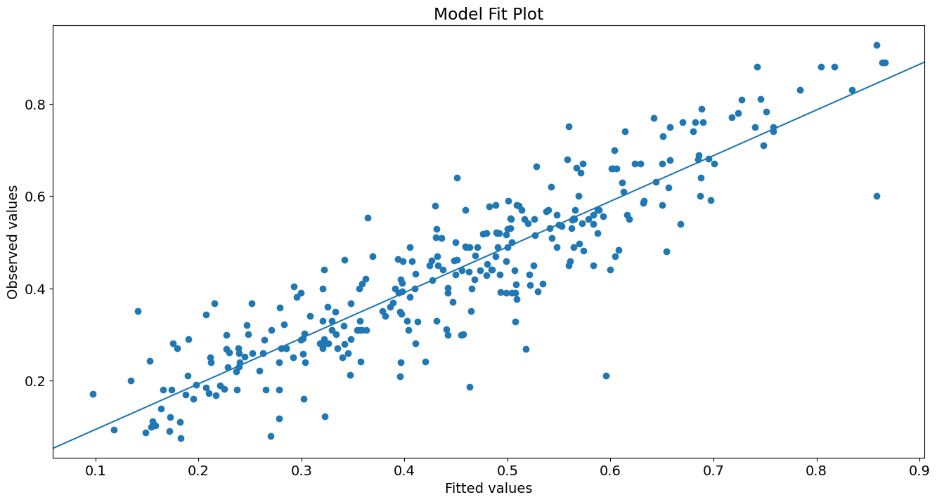
yhat 対 y のプロット
[12]:
from statsmodels.graphics.api import abline_plot
[13]:
fig, ax = plt.subplots()
ax.scatter(yhat, y)
line_fit = sm.OLS(y, sm.add_constant(yhat, prepend=True)).fit()
abline_plot(model_results=line_fit, ax=ax)


ax.set_title('Model Fit Plot')
ax.set_ylabel('Observed values')
ax.set_xlabel('Fitted values');
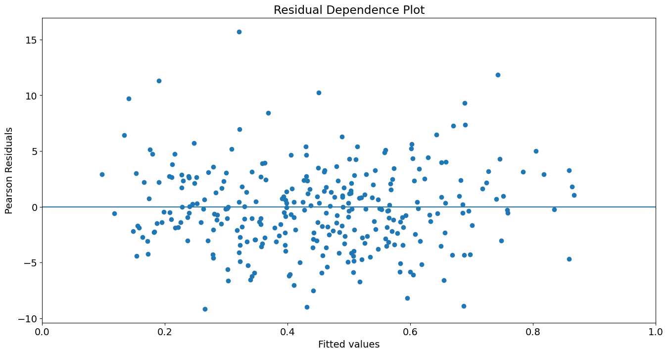
yhat 対ピアソン残差のプロット
[14]:
fig, ax = plt.subplots()

ax.scatter(yhat, res.resid_pearson)
ax.hlines(0, 0, 1)
ax.set_xlim(0, 1)
ax.set_title('Residual Dependence Plot')
ax.set_ylabel('Pearson Residuals')
ax.set_xlabel('Fitted values')
[14]:
Text(0.5, 0, 'Fitted values')
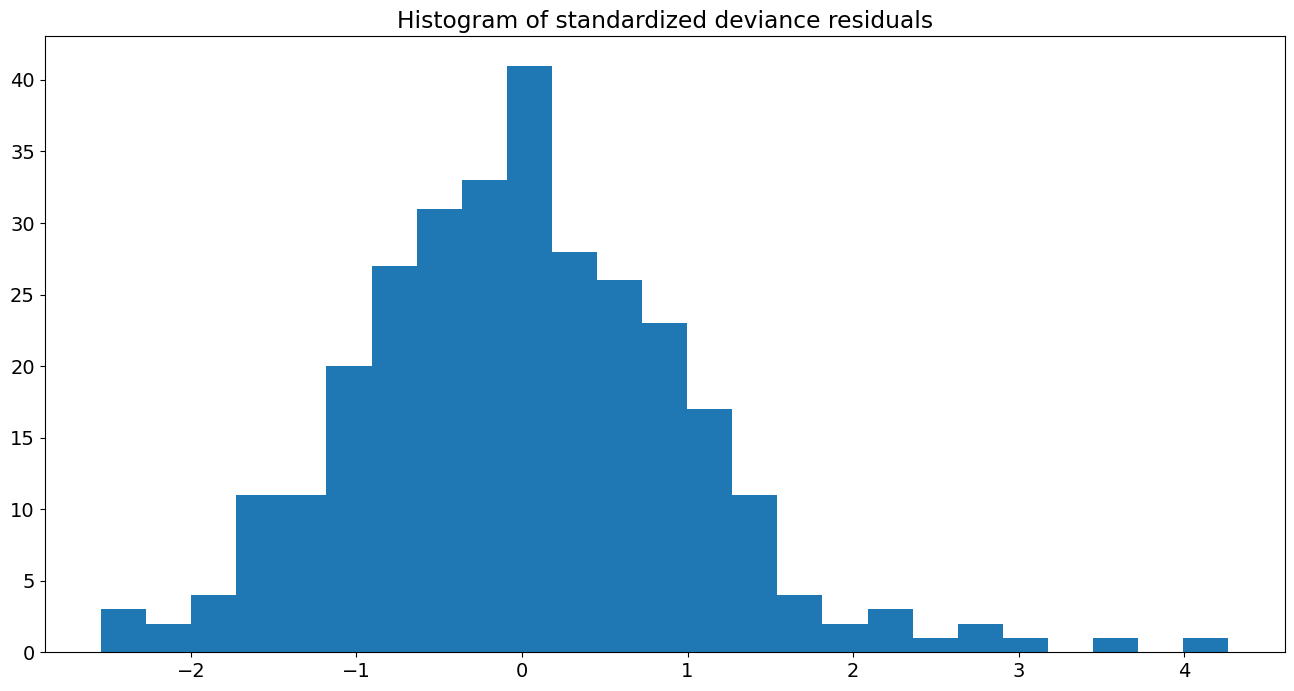
標準化された逸脱度残差のヒストグラム
[15]:
from scipy import stats

fig, ax = plt.subplots()

resid = res.resid_deviance.copy()
resid_std = stats.zscore(resid)
ax.hist(resid_std, bins=25)
ax.set_title('Histogram of standardized deviance residuals');
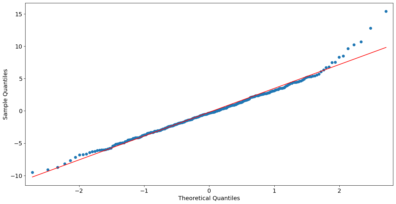
逸脱度残差の QQ プロット
[16]:
from statsmodels import graphics
graphics.gofplots.qqplot(resid, line='r')
[16]:

GLM: 比例カウント応答のためのガンマ
スコットランド議会投票データの読み込み
上記の例では、`NOTE` 属性を出力して Star98 データセットについて学習しました。 statsmodels データセットには、他の役立つ情報も付属しています。例えば
[17]:
print(sm.datasets.scotland.DESCRLONG)
This data is based on the example in Gill and describes the proportion of
voters who voted Yes to grant the Scottish Parliament taxation powers.
The data are divided into 32 council districts.  This example's explanatory
variables include the amount of council tax collected in pounds sterling as
of April 1997 per two adults before adjustments, the female percentage of
total claims for unemployment benefits as of January, 1998, the standardized
mortality rate (UK is 100), the percentage of labor force participation,
regional GDP, the percentage of children aged 5 to 15, and an interaction term
between female unemployment and the council tax.

The original source files and variable information are included in
/scotland/src/
データを読み込み、外生変数に定数を追加します
[18]:
data2 = sm.datasets.scotland.load()
data2.exog = sm.add_constant(data2.exog, prepend=False)
print(data2.exog.head())
print(data2.endog.head())
   COUTAX  UNEMPF    MOR   ACT      GDP   AGE  COUTAX_FEMALEUNEMP  const
0   712.0    21.0  105.0  82.4  13566.0  12.3             14952.0    1.0
1   643.0    26.5   97.0  80.2  13566.0  15.3             17039.5    1.0
2   679.0    28.3  113.0  86.3   9611.0  13.9             19215.7    1.0
3   801.0    27.1  109.0  80.4   9483.0  13.6             21707.1    1.0
4   753.0    22.0  115.0  64.7   9265.0  14.6             16566.0    1.0
0    60.3
1    52.3
2    53.4
3    57.0
4    68.7
Name: YES, dtype: float64
モデルの適合とサマリー
[19]:
glm_gamma = sm.GLM(data2.endog, data2.exog, family=sm.families.Gamma(sm.families.links.Log()))
glm_results = glm_gamma.fit()
print(glm_results.summary())
                 Generalized Linear Model Regression Results
==============================================================================
Dep. Variable:                    YES   No. Observations:                   32
Model:                            GLM   Df Residuals:                       24
Model Family:                   Gamma   Df Model:                            7
Link Function:                    Log   Scale:                       0.0035927
Method:                          IRLS   Log-Likelihood:                -83.110
Date:                Thu, 03 Oct 2024   Deviance:                     0.087988
Time:                        15:46:29   Pearson chi2:                   0.0862
No. Iterations:                     7   Pseudo R-squ. (CS):             0.9797
Covariance Type:            nonrobust
======================================================================================
                         coef    std err          z      P>|z|      [0.025      0.975]
--------------------------------------------------------------------------------------
COUTAX                -0.0024      0.001     -2.466      0.014      -0.004      -0.000
UNEMPF                -0.1005      0.031     -3.269      0.001      -0.161      -0.040
MOR                    0.0048      0.002      2.946      0.003       0.002       0.008
ACT                   -0.0067      0.003     -2.534      0.011      -0.012      -0.002
GDP                 8.173e-06   7.19e-06      1.136      0.256   -5.93e-06    2.23e-05
AGE                    0.0298      0.015      2.009      0.045       0.001       0.059
COUTAX_FEMALEUNEMP     0.0001   4.33e-05      2.724      0.006    3.31e-05       0.000
const                  5.6581      0.680      8.318      0.000       4.325       6.991
======================================================================================
GLM: 非正準リンクを持つガウス分布
人工データ
[20]:
nobs2 = 100
x = np.arange(nobs2)
np.random.seed(54321)
X = np.column_stack((x,x**2))
X = sm.add_constant(X, prepend=False)
lny = np.exp(-(.03*x + .0001*x**2 - 1.0)) + .001 * np.random.rand(nobs2)
適合とサマリー (人工データ)
[21]:
gauss_log = sm.GLM(lny, X, family=sm.families.Gaussian(sm.families.links.Log()))
gauss_log_results = gauss_log.fit()
print(gauss_log_results.summary())
                 Generalized Linear Model Regression Results
==============================================================================
Dep. Variable:                      y   No. Observations:                  100
Model:                            GLM   Df Residuals:                       97
Model Family:                Gaussian   Df Model:                            2
Link Function:                    Log   Scale:                      1.0531e-07
Method:                          IRLS   Log-Likelihood:                 662.92
Date:                Thu, 03 Oct 2024   Deviance:                   1.0215e-05
Time:                        15:46:29   Pearson chi2:                 1.02e-05
No. Iterations:                     7   Pseudo R-squ. (CS):              1.000
Covariance Type:            nonrobust
==============================================================================
                 coef    std err          z      P>|z|      [0.025      0.975]
------------------------------------------------------------------------------
x1            -0.0300    5.6e-06  -5361.316      0.000      -0.030      -0.030
x2         -9.939e-05   1.05e-07   -951.091      0.000   -9.96e-05   -9.92e-05
const          1.0003   5.39e-05   1.86e+04      0.000       1.000       1.000
==============================================================================
最終更新日: 2024年10月03日