カーネル密度推定¶

カーネル密度推定とは、*カーネル関数* \(K(u)\) を使用して未知の確率密度関数を推定するプロセスです。ヒストグラムは、やや恣意的な領域内のデータポイントの数をカウントしますが、カーネル密度推定値は、すべてのデータポイントにおけるカーネル関数の合計として定義される関数です。カーネル関数は通常、以下の特性を示します。

\(K(u) = K(-u)\) となるような対称性。
\(\int_{-\infty}^{\infty} K(u) \ du = 1\) となるような正規化。
\(u > 0\) のとき \(K'(u) < 0\) となるような単調減少。
\(\mathrm{E}[K] = 0\) となるような、ゼロに等しい期待値。

カーネル密度推定の詳細については、例えば Wikipedia - カーネル密度推定を参照してください。

単変量カーネル密度推定量は、sm.nonparametric.KDEUnivariate に実装されています。この例では、以下を示します。

基本的な使用方法、推定量のフィッティング方法。
bw 引数を使用してカーネルの帯域幅を変更することの影響。
kernel 引数を使用して利用可能な様々なカーネル関数。

[1]:

%matplotlib inline
import numpy as np
from scipy import stats
import statsmodels.api as sm
import matplotlib.pyplot as plt
from statsmodels.distributions.mixture_rvs import mixture_rvs

単変量の例¶

[2]:

np.random.seed(12345)  # Seed the random number generator for reproducible results

双峰分布を作成します。位置が -1 と 1 の2つの正規分布の混合です。

[3]:

# Location, scale and weight for the two distributions
dist1_loc, dist1_scale, weight1 = -1, 0.5, 0.25
dist2_loc, dist2_scale, weight2 = 1, 0.5, 0.75

# Sample from a mixture of distributions
obs_dist = mixture_rvs(
    prob=[weight1, weight2],
    size=250,
    dist=[stats.norm, stats.norm],
    kwargs=(
        dict(loc=dist1_loc, scale=dist1_scale),
        dict(loc=dist2_loc, scale=dist2_scale),
    ),
)

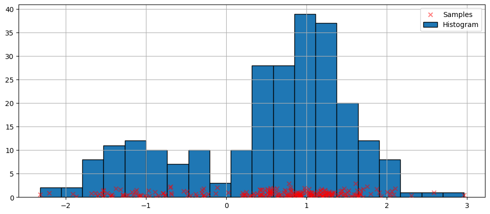
密度推定のための最も単純なノンパラメトリック手法はヒストグラムです。

[4]:

fig = plt.figure(figsize=(12, 5))
ax = fig.add_subplot(111)

# Scatter plot of data samples and histogram
ax.scatter(
    obs_dist,
    np.abs(np.random.randn(obs_dist.size)),
    zorder=15,
    color="red",
    marker="x",
    alpha=0.5,
    label="Samples",
)
lines = ax.hist(obs_dist, bins=20, edgecolor="k", label="Histogram")

ax.legend(loc="best")
ax.grid(True, zorder=-5)

../../../_images/examples_notebooks_generated_kernel_density_7_0.png

デフォルト引数でのフィッティング¶

上記のヒストグラムは不連続です。連続確率密度関数を計算するために、カーネル密度推定を使用できます。

KDEUnivariate を使用して、単変量カーネル密度推定量を初期化します。

[5]:

kde = sm.nonparametric.KDEUnivariate(obs_dist)
kde.fit()  # Estimate the densities

[5]:

<statsmodels.nonparametric.kde.KDEUnivariate at 0x7fed558239a0>

フィットの図と、真の分布を示します。

[6]:

fig = plt.figure(figsize=(12, 5))
ax = fig.add_subplot(111)

# Plot the histogram
ax.hist(
    obs_dist,
    bins=20,
    density=True,
    label="Histogram from samples",
    zorder=5,
    edgecolor="k",
    alpha=0.5,
)

# Plot the KDE as fitted using the default arguments
ax.plot(kde.support, kde.density, lw=3, label="KDE from samples", zorder=10)

# Plot the true distribution
true_values = (
    stats.norm.pdf(loc=dist1_loc, scale=dist1_scale, x=kde.support) * weight1
    + stats.norm.pdf(loc=dist2_loc, scale=dist2_scale, x=kde.support) * weight2
)
ax.plot(kde.support, true_values, lw=3, label="True distribution", zorder=15)

# Plot the samples
ax.scatter(
    obs_dist,
    np.abs(np.random.randn(obs_dist.size)) / 40,
    marker="x",
    color="red",
    zorder=20,
    label="Samples",
    alpha=0.5,
)

ax.legend(loc="best")
ax.grid(True, zorder=-5)

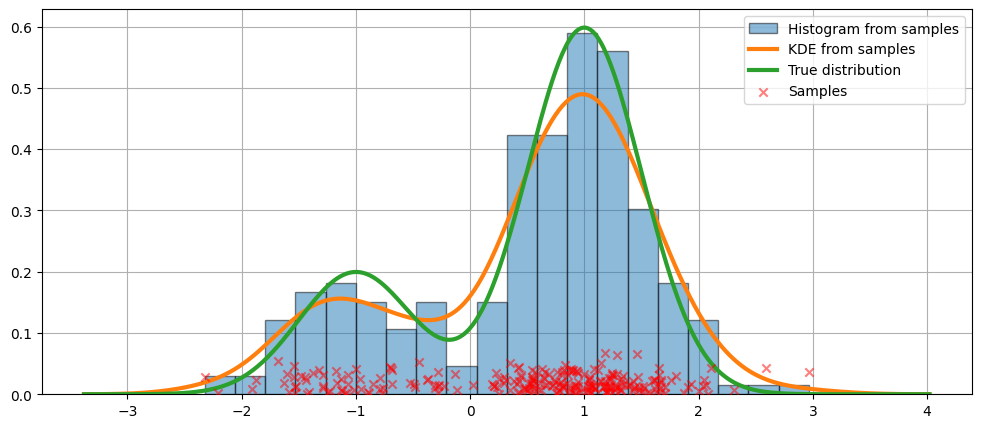
../../../_images/examples_notebooks_generated_kernel_density_12_0.png

上記のコードでは、デフォルトの引数が使用されました。カーネルの帯域幅を変更することもできます。次に示します。

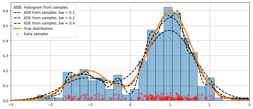
`bw` 引数を使用した帯域幅の変更¶

カーネルの帯域幅は、bw 引数を使用して調整できます。次の例では、bw=0.2 の帯域幅がデータによく適合しているようです。

[7]:

fig = plt.figure(figsize=(12, 5))
ax = fig.add_subplot(111)

# Plot the histogram
ax.hist(
    obs_dist,
    bins=25,
    label="Histogram from samples",
    zorder=5,
    edgecolor="k",
    density=True,
    alpha=0.5,
)

# Plot the KDE for various bandwidths
for bandwidth in [0.1, 0.2, 0.4]:
    kde.fit(bw=bandwidth)  # Estimate the densities
    ax.plot(
        kde.support,
        kde.density,
        "--",
        lw=2,
        color="k",
        zorder=10,
        label="KDE from samples, bw = {}".format(round(bandwidth, 2)),
    )

# Plot the true distribution
ax.plot(kde.support, true_values, lw=3, label="True distribution", zorder=15)

# Plot the samples
ax.scatter(
    obs_dist,
    np.abs(np.random.randn(obs_dist.size)) / 50,
    marker="x",
    color="red",
    zorder=20,
    label="Data samples",
    alpha=0.5,
)

ax.legend(loc="best")
ax.set_xlim([-3, 3])
ax.grid(True, zorder=-5)

../../../_images/examples_notebooks_generated_kernel_density_16_0.png

カーネル関数の比較¶

上記の例では、ガウスカーネルが使用されました。他にもいくつかのカーネルが利用可能です。

[8]:

from statsmodels.nonparametric.kde import kernel_switch

list(kernel_switch.keys())

[8]:

['gau', 'epa', 'uni', 'tri', 'biw', 'triw', 'cos', 'cos2', 'tric']

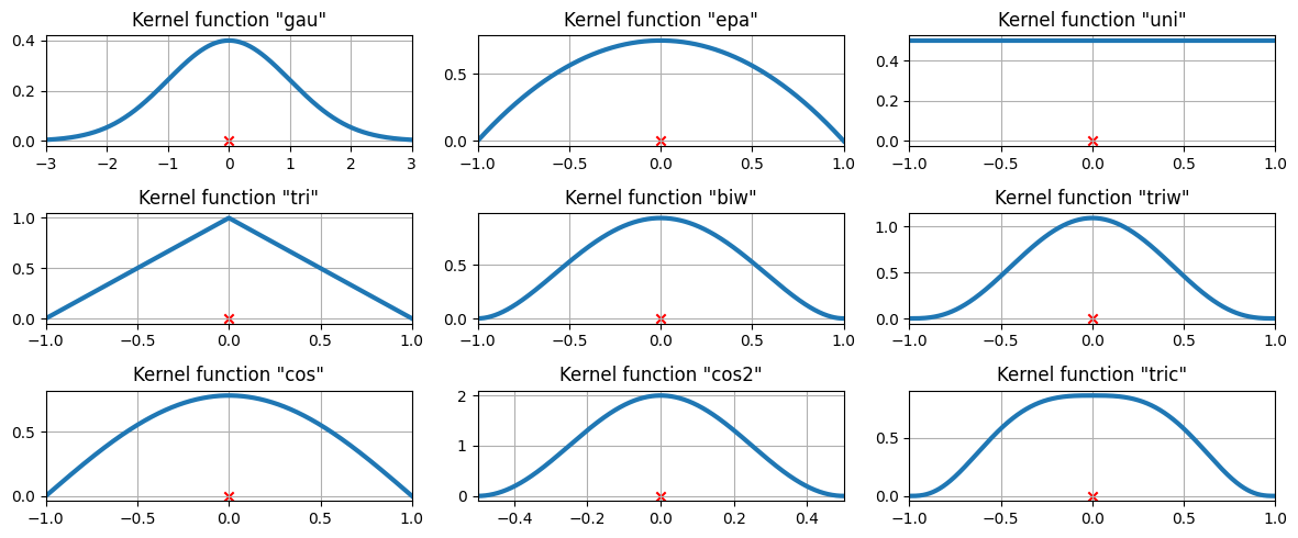
利用可能なカーネル関数¶

[9]:

# Create a figure
fig = plt.figure(figsize=(12, 5))

# Enumerate every option for the kernel
for i, (ker_name, ker_class) in enumerate(kernel_switch.items()):

    # Initialize the kernel object
    kernel = ker_class()

    # Sample from the domain
    domain = kernel.domain or [-3, 3]
    x_vals = np.linspace(*domain, num=2 ** 10)
    y_vals = kernel(x_vals)

    # Create a subplot, set the title
    ax = fig.add_subplot(3, 3, i + 1)
    ax.set_title('Kernel function "{}"'.format(ker_name))
    ax.plot(x_vals, y_vals, lw=3, label="{}".format(ker_name))
    ax.scatter([0], [0], marker="x", color="red")
    plt.grid(True, zorder=-5)
    ax.set_xlim(domain)

plt.tight_layout()

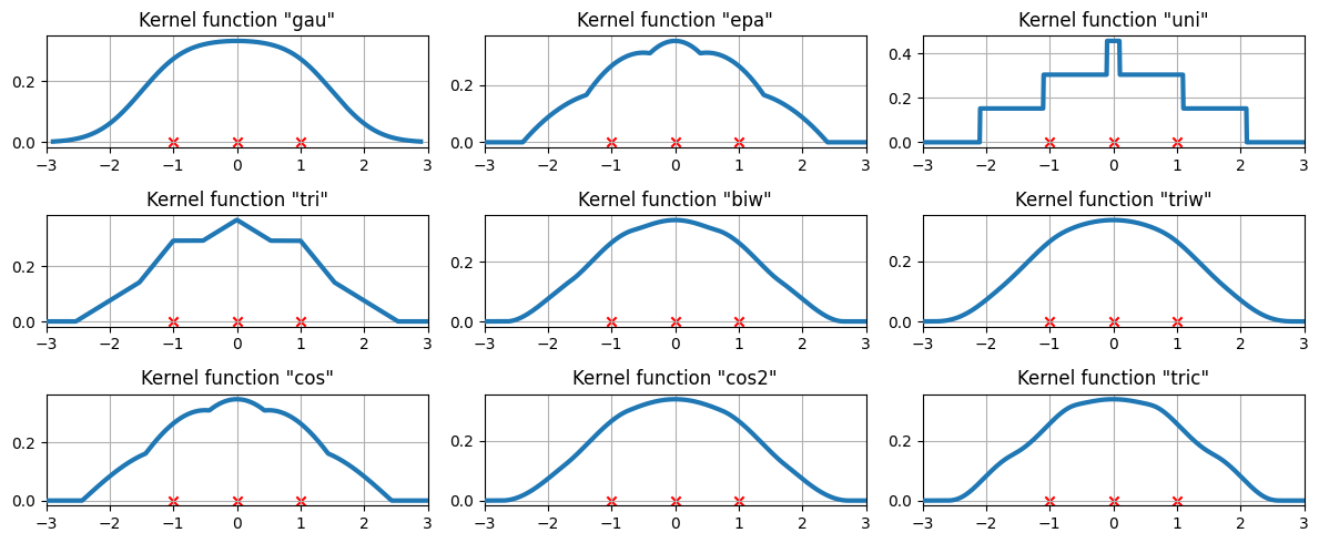
../../../_images/examples_notebooks_generated_kernel_density_21_0.png

3つのデータポイントにおける利用可能なカーネル関数¶

等間隔に配置された3つのデータポイントに、カーネル密度推定値がどのように適合するかを調べます。

[10]:

# Create three equidistant points
data = np.linspace(-1, 1, 3)
kde = sm.nonparametric.KDEUnivariate(data)

# Create a figure
fig = plt.figure(figsize=(12, 5))

# Enumerate every option for the kernel
for i, kernel in enumerate(kernel_switch.keys()):

    # Create a subplot, set the title
    ax = fig.add_subplot(3, 3, i + 1)
    ax.set_title('Kernel function "{}"'.format(kernel))

    # Fit the model (estimate densities)
    kde.fit(kernel=kernel, fft=False, gridsize=2 ** 10)

    # Create the plot
    ax.plot(kde.support, kde.density, lw=3, label="KDE from samples", zorder=10)
    ax.scatter(data, np.zeros_like(data), marker="x", color="red")
    plt.grid(True, zorder=-5)
    ax.set_xlim([-3, 3])

plt.tight_layout()

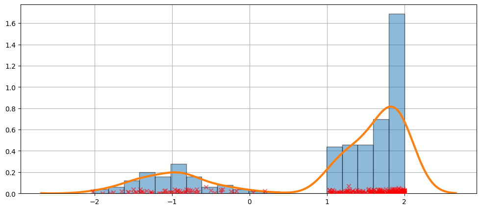
../../../_images/examples_notebooks_generated_kernel_density_24_0.png

より難しいケース¶

フィットが常に完璧であるとは限りません。より難しいケースについては、以下の例を参照してください。

[11]:

obs_dist = mixture_rvs(
    [0.25, 0.75],
    size=250,
    dist=[stats.norm, stats.beta],
    kwargs=(dict(loc=-1, scale=0.5), dict(loc=1, scale=1, args=(1, 0.5))),
)

[12]:

kde = sm.nonparametric.KDEUnivariate(obs_dist)
kde.fit()

[12]:

<statsmodels.nonparametric.kde.KDEUnivariate at 0x7fed52347940>

[13]:

fig = plt.figure(figsize=(12, 5))
ax = fig.add_subplot(111)
ax.hist(obs_dist, bins=20, density=True, edgecolor="k", zorder=4, alpha=0.5)
ax.plot(kde.support, kde.density, lw=3, zorder=7)
# Plot the samples
ax.scatter(
    obs_dist,
    np.abs(np.random.randn(obs_dist.size)) / 50,
    marker="x",
    color="red",
    zorder=20,
    label="Data samples",
    alpha=0.5,
)
ax.grid(True, zorder=-5)

../../../_images/examples_notebooks_generated_kernel_density_28_0.png

KDEは分布です¶

KDEは分布であるため、以下のような属性やメソッドにアクセスできます。

エントロピー
評価
cdf
icdf
sf
累積ハザード

[14]:

obs_dist = mixture_rvs(
    [0.25, 0.75],
    size=1000,
    dist=[stats.norm, stats.norm],
    kwargs=(dict(loc=-1, scale=0.5), dict(loc=1, scale=0.5)),
)
kde = sm.nonparametric.KDEUnivariate(obs_dist)
kde.fit(gridsize=2 ** 10)

[14]:

<statsmodels.nonparametric.kde.KDEUnivariate at 0x7fed535c1c00>

[15]:

kde.entropy

[15]:

1.314324140492138

[16]:

kde.evaluate(-1)

[16]:

array([0.18085886])

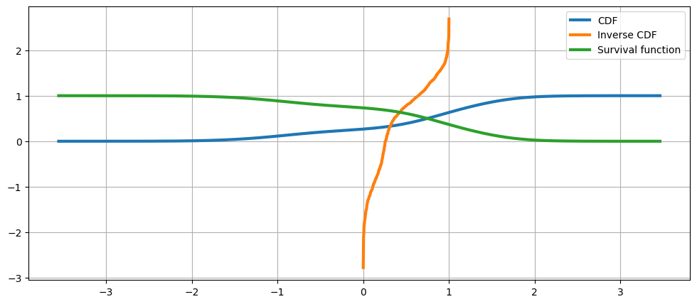
累積分布関数、その逆関数、および生存関数¶

[17]:

fig = plt.figure(figsize=(12, 5))
ax = fig.add_subplot(111)

ax.plot(kde.support, kde.cdf, lw=3, label="CDF")
ax.plot(np.linspace(0, 1, num=kde.icdf.size), kde.icdf, lw=3, label="Inverse CDF")
ax.plot(kde.support, kde.sf, lw=3, label="Survival function")
ax.legend(loc="best")
ax.grid(True, zorder=-5)

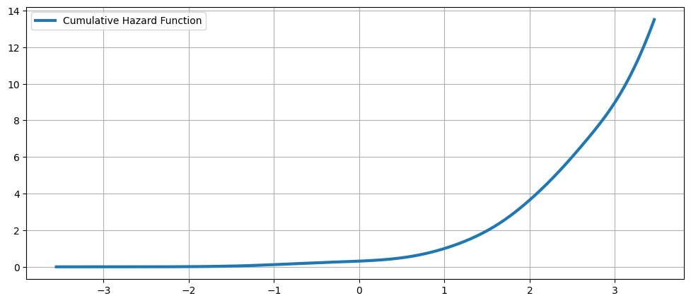
../../../_images/examples_notebooks_generated_kernel_density_34_0.png

累積ハザード関数¶

[18]:

fig = plt.figure(figsize=(12, 5))
ax = fig.add_subplot(111)
ax.plot(kde.support, kde.cumhazard, lw=3, label="Cumulative Hazard Function")
ax.legend(loc="best")
ax.grid(True, zorder=-5)

../../../_images/examples_notebooks_generated_kernel_density_36_0.png

最終更新日: 2024年10月3日