予測 (サンプル外)
[1]:
%matplotlib inline
[2]:
import numpy as np
import matplotlib.pyplot as plt

import statsmodels.api as sm

plt.rc("figure", figsize=(16, 8))
plt.rc("font", size=14)
人工データ
[3]:
nsample = 50
sig = 0.25
x1 = np.linspace(0, 20, nsample)
X = np.column_stack((x1, np.sin(x1), (x1 - 5) ** 2))
X = sm.add_constant(X)
beta = [5.0, 0.5, 0.5, -0.02]
y_true = np.dot(X, beta)
y = y_true + sig * np.random.normal(size=nsample)
推定
[4]:
olsmod = sm.OLS(y, X)
olsres = olsmod.fit()
print(olsres.summary())
                            OLS Regression Results
==============================================================================
Dep. Variable:                      y   R-squared:                       0.980
Model:                            OLS   Adj. R-squared:                  0.979
Method:                 Least Squares   F-statistic:                     767.8
Date:                Thu, 03 Oct 2024   Prob (F-statistic):           2.80e-39
Time:                        15:50:37   Log-Likelihood:                -3.6609
No. Observations:                  50   AIC:                             15.32
Df Residuals:                      46   BIC:                             22.97
Df Model:                           3
Covariance Type:            nonrobust
==============================================================================
                 coef    std err          t      P>|t|      [0.025      0.975]
------------------------------------------------------------------------------
const          5.0304      0.093     54.373      0.000       4.844       5.217
x1             0.5002      0.014     35.058      0.000       0.471       0.529
x2             0.5011      0.056      8.934      0.000       0.388       0.614
x3            -0.0201      0.001    -16.012      0.000      -0.023      -0.018
==============================================================================
Omnibus:                        2.155   Durbin-Watson:                   1.847
Prob(Omnibus):                  0.340   Jarque-Bera (JB):                2.068
Skew:                          -0.462   Prob(JB):                        0.356
Kurtosis:                       2.630   Cond. No.                         221.
==============================================================================

Notes:
[1] Standard Errors assume that the covariance matrix of the errors is correctly specified.
サンプル内予測
[5]:
ypred = olsres.predict(X)
print(ypred)
[ 4.52892208  5.01052175  5.45275967  5.82832671  6.11976948  6.32235784
  6.44486207  6.50811191  6.54157432  6.57851213  6.65051904  6.7823289
  6.98775197  7.26740594  7.60861448  7.98748987  8.37285773  8.73137887
  9.03302681  9.25602105  9.39040558  9.43968456  9.42024665  9.35867239
  9.28736706  9.23923662  9.24228135  9.31499546  9.46332857  9.67970819
  9.94428385 10.2281885  10.49828128 10.72259244 10.87557591 10.94230645
 10.9209318  10.82297701 10.67145093 10.49706588 10.33319174 10.21037335
 10.15131209 10.1671361  10.25557197 10.40131825 10.57855941 10.75520731
 10.89817315 10.97880387]
説明変数 Xnew の新しいサンプルを作成、予測、プロット
[6]:
x1n = np.linspace(20.5, 25, 10)
Xnew = np.column_stack((x1n, np.sin(x1n), (x1n - 5) ** 2))
Xnew = sm.add_constant(Xnew)
ynewpred = olsres.predict(Xnew)  # predict out of sample
print(ynewpred)
[10.96503747 10.81894524 10.56017815 10.23351824  9.89791447  9.61204991
  9.4199741   9.34031818  9.36173334  9.44566941]
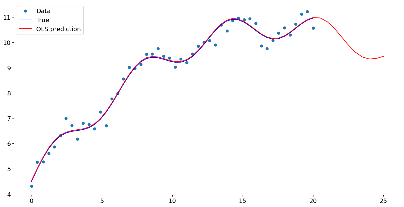
プロットの比較
[7]:
import matplotlib.pyplot as plt

fig, ax = plt.subplots()
ax.plot(x1, y, "o", label="Data")
ax.plot(x1, y_true, "b-", label="True")
ax.plot(np.hstack((x1, x1n)), np.hstack((ypred, ynewpred)), "r", label="OLS prediction")
ax.legend(loc="best")
[7]:
<matplotlib.legend.Legend at 0x7f30514b3fd0>
数式による予測
数式を使用すると、推定と予測のどちらも大幅に簡単になります
[8]:
from statsmodels.formula.api import ols

data = {"x1": x1, "y": y}

res = ols("y ~ x1 + np.sin(x1) + I((x1-5)**2)", data=data).fit()
I を使用して、単位変換を使用することを示します。つまるところ、**2 の使用による拡張のトリックは必要ありません
[9]:
res.params
[9]:
Intercept           5.030411
x1                  0.500216
np.sin(x1)          0.501093
I((x1 - 5) ** 2)   -0.020060
dtype: float64
変数は単一のみを指定する必要があり、変換後の右辺の変数は自動的に取得されます
[10]:
res.predict(exog=dict(x1=x1n))
[10]:
0    10.965037
1    10.818945
2    10.560178
3    10.233518
4     9.897914
5     9.612050
6     9.419974
7     9.340318
8     9.361733
9     9.445669
dtype: float64
最終更新: 2024 年 10 月 3 日