statsmodelsにおける予測
このノートブックでは、statsmodelsにおける時系列モデルを用いた予測について説明します。
注意: このノートブックは、状態空間モデルクラスにのみ適用されます。
sm.tsa.SARIMAXsm.tsa.UnobservedComponentssm.tsa.VARMAXsm.tsa.DynamicFactor
[1]:
%matplotlib inline

import numpy as np
import pandas as pd
import statsmodels.api as sm
import matplotlib.pyplot as plt

macrodata = sm.datasets.macrodata.load_pandas().data
macrodata.index = pd.period_range('1959Q1', '2009Q3', freq='Q')
基本例
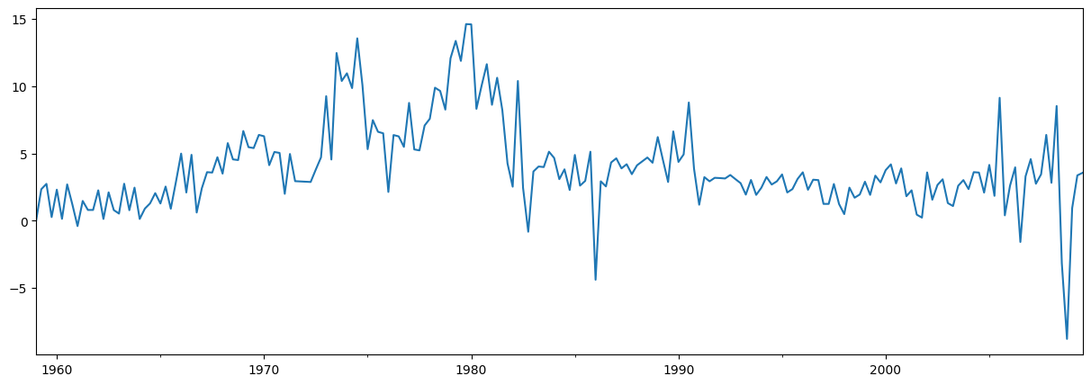
簡単な例として、AR(1)モデルを用いてインフレ率を予測します。予測の前に、系列を見てみましょう。
[2]:
endog = macrodata['infl']
endog.plot(figsize=(15, 5))
[2]:
<Axes: >
モデルの構築と推定
次のステップは、予測に使用する計量経済モデルを定式化することです。この場合、statsmodelsのSARIMAXクラスを介してAR(1)モデルを使用します。
モデルを構築した後、そのパラメータを推定する必要があります。これは、fitメソッドを使用して行います。summaryメソッドは、結果を示すいくつかの便利なテーブルを作成します。
[3]:
# Construct the model
mod = sm.tsa.SARIMAX(endog, order=(1, 0, 0), trend='c')
# Estimate the parameters
res = mod.fit()

print(res.summary())
RUNNING THE L-BFGS-B CODE

           * * *

Machine precision = 2.220D-16
 N =            3     M =           10

At X0         0 variables are exactly at the bounds

At iterate    0    f=  2.32873D+00    |proj g|=  8.23649D-03

At iterate    5    f=  2.32864D+00    |proj g|=  1.41994D-03

           * * *

Tit   = total number of iterations
Tnf   = total number of function evaluations
Tnint = total number of segments explored during Cauchy searches
Skip  = number of BFGS updates skipped
Nact  = number of active bounds at final generalized Cauchy point
Projg = norm of the final projected gradient
F     = final function value

           * * *

   N    Tit     Tnf  Tnint  Skip  Nact     Projg        F
    3      8     10      1     0     0   5.820D-06   2.329D+00
  F =   2.3286389358138617

CONVERGENCE: NORM_OF_PROJECTED_GRADIENT_<=_PGTOL
                               SARIMAX Results
==============================================================================
Dep. Variable:                   infl   No. Observations:                  203
Model:               SARIMAX(1, 0, 0)   Log Likelihood                -472.714
Date:                Thu, 03 Oct 2024   AIC                            951.427
Time:                        16:07:30   BIC                            961.367
Sample:                    03-31-1959   HQIC                           955.449
                         - 09-30-2009
Covariance Type:                  opg
==============================================================================
                 coef    std err          z      P>|z|      [0.025      0.975]
------------------------------------------------------------------------------
intercept      1.3962      0.254      5.488      0.000       0.898       1.895
ar.L1          0.6441      0.039     16.482      0.000       0.568       0.721
sigma2         6.1519      0.397     15.487      0.000       5.373       6.930
===================================================================================
Ljung-Box (L1) (Q):                   8.43   Jarque-Bera (JB):                68.45
Prob(Q):                              0.00   Prob(JB):                         0.00
Heteroskedasticity (H):               1.47   Skew:                            -0.22
Prob(H) (two-sided):                  0.12   Kurtosis:                         5.81
===================================================================================

Warnings:
[1] Covariance matrix calculated using the outer product of gradients (complex-step).
This problem is unconstrained.
予測
サンプル外の予測は、結果オブジェクトからforecastまたはget_forecastメソッドを使用して生成されます。
forecastメソッドは、点予測のみを提供します。
[4]:
# The default is to get a one-step-ahead forecast:
print(res.forecast())
2009Q4    3.68921
Freq: Q-DEC, dtype: float64
get_forecastメソッドはより一般的であり、信頼区間の構築も可能です。
[5]:
# Here we construct a more complete results object.
fcast_res1 = res.get_forecast()

# Most results are collected in the `summary_frame` attribute.
# Here we specify that we want a confidence level of 90%
print(fcast_res1.summary_frame(alpha=0.10))
infl       mean   mean_se  mean_ci_lower  mean_ci_upper
2009Q4  3.68921  2.480302      -0.390523       7.768943
デフォルトの信頼水準は95%ですが、これはalphaパラメータを設定することで制御できます。信頼水準は\((1 - \alpha) \times 100\%\)として定義されます。上記の例では、alpha=0.10を使用して、90%の信頼水準を指定しました。
予測数の指定
forecastとget_forecastの両方の関数は、いくつの予測ステップが必要かを示す単一の引数を受け入れます。この引数の1つのオプションは、常に必要なステップ数を表す整数を指定することです。
[6]:
print(res.forecast(steps=2))
2009Q4    3.689210
2010Q1    3.772434
Freq: Q-DEC, Name: predicted_mean, dtype: float64
[7]:
fcast_res2 = res.get_forecast(steps=2)
# Note: since we did not specify the alpha parameter, the
# confidence level is at the default, 95%
print(fcast_res2.summary_frame())
infl        mean   mean_se  mean_ci_lower  mean_ci_upper
2009Q4  3.689210  2.480302      -1.172092       8.550512
2010Q1  3.772434  2.950274      -2.009996       9.554865
ただし、データに頻度が定義されたPandasインデックスが含まれている場合(詳細については、最後のインデックスのセクションを参照)、代わりに予測を生成する日付を指定できます。
[8]:
print(res.forecast('2010Q2'))
2009Q4    3.689210
2010Q1    3.772434
2010Q2    3.826039
Freq: Q-DEC, Name: predicted_mean, dtype: float64
[9]:
fcast_res3 = res.get_forecast('2010Q2')
print(fcast_res3.summary_frame())
infl        mean   mean_se  mean_ci_lower  mean_ci_upper
2009Q4  3.689210  2.480302      -1.172092       8.550512
2010Q1  3.772434  2.950274      -2.009996       9.554865
2010Q2  3.826039  3.124571      -2.298008       9.950087
データ、予測、信頼区間のプロット
多くの場合、データ、予測、信頼区間をプロットすると便利です。これを行うには多くの方法がありますが、ここに1つの例を示します。
[10]:
fig, ax = plt.subplots(figsize=(15, 5))

# Plot the data (here we are subsetting it to get a better look at the forecasts)
endog.loc['1999':].plot(ax=ax)

# Construct the forecasts
fcast = res.get_forecast('2011Q4').summary_frame()
fcast['mean'].plot(ax=ax, style='k--')
ax.fill_between(fcast.index, fcast['mean_ci_lower'], fcast['mean_ci_upper'], color='k', alpha=0.1);
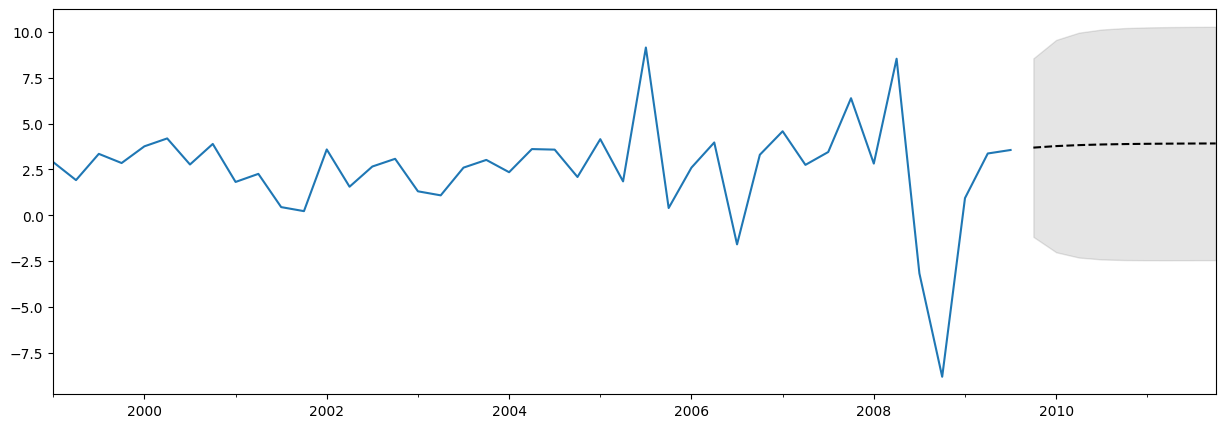
予測から期待されることについての注意
上記の予測は、ほぼ直線であるため、それほど印象的ではないかもしれません。これは、非常に単純な単変量予測モデルであるためです。それでも、これらの単純な予測モデルは非常に競争力がある可能性があることに留意してください。
予測 vs 予測
結果オブジェクトには、サンプル内適合値とサンプル外予測の両方を可能にする2つのメソッドも含まれています。それらは、predictとget_predictionです。predictメソッドは点予測のみを返しますが(forecastと同様)、get_predictionメソッドは追加の結果も返します(get_forecastと同様)。
一般に、サンプル外予測に興味がある場合は、forecastとget_forecastメソッドにこだわる方が簡単です。
クロスバリデーション
注意: このセクションで使用されている関数のいくつかは、statsmodels v0.11.0で初めて導入されました。
一般的なユースケースは、次のプロセスを使用して再帰的にhステップ先の予測を実行することにより、予測方法をクロスバリデーションすることです。
トレーニングサンプルにモデルパラメータを適合させる
そのサンプルの終わりからhステップ先の予測を生成する
テストデータセットと予測を比較して、エラー率を計算する
サンプルを展開して次の観測値を含め、繰り返す
エコノミストは、これを疑似サンプル外予測評価演習、または時系列クロスバリデーションと呼ぶことがあります。
例
上記のインフレデータセットを使用して、この種の非常に簡単な演習を実施します。完全なデータセットには203個の観測値が含まれており、説明のために最初の80%をトレーニングサンプルとして使用し、1ステップ先の予測のみを考慮します。
上記の手順の単一反復は、次のようになります。
[11]:
# Step 1: fit model parameters w/ training sample
training_obs = int(len(endog) * 0.8)

training_endog = endog[:training_obs]
training_mod = sm.tsa.SARIMAX(
    training_endog, order=(1, 0, 0), trend='c')
training_res = training_mod.fit()

# Print the estimated parameters
print(training_res.params)
RUNNING THE L-BFGS-B CODE

           * * *

Machine precision = 2.220D-16
 N =            3     M =           10

At X0         0 variables are exactly at the bounds

At iterate    0    f=  2.23132D+00    |proj g|=  1.09171D-02

At iterate    5    f=  2.23109D+00    |proj g|=  3.93608D-05

           * * *

Tit   = total number of iterations
Tnf   = total number of function evaluations
Tnint = total number of segments explored during Cauchy searches
Skip  = number of BFGS updates skipped
Nact  = number of active bounds at final generalized Cauchy point
Projg = norm of the final projected gradient
F     = final function value

           * * *

   N    Tit     Tnf  Tnint  Skip  Nact     Projg        F
    3      6      8      1     0     0   7.066D-07   2.231D+00
  F =   2.2310884444664758

CONVERGENCE: NORM_OF_PROJECTED_GRADIENT_<=_PGTOL
intercept    1.162076
ar.L1        0.724242
sigma2       5.051600
dtype: float64
This problem is unconstrained.
[12]:
# Step 2: produce one-step-ahead forecasts
fcast = training_res.forecast()

# Step 3: compute root mean square forecasting error
true = endog.reindex(fcast.index)
error = true - fcast

# Print out the results
print(pd.concat([true.rename('true'),
                 fcast.rename('forecast'),
                 error.rename('error')], axis=1))
        true  forecast    error
1999Q3  3.35   2.55262  0.79738
別の観測値を追加するには、appendまたはextend結果メソッドを使用できます。どちらのメソッドも同じ予測を生成できますが、利用可能な他の結果が異なります。
appendは、より完全なメソッドです。常にすべてのトレーニング観測値の結果を保存し、オプションで新しい観測値を指定してモデルパラメータを再適合させることができます(デフォルトはパラメータを再適合させ*ない*ことに注意してください)。extendは、トレーニングサンプルが非常に大きい場合に役立つ高速なメソッドです。*新しい*観測値の結果のみを保存し、モデルパラメータの再適合は許可しません(つまり、前のサンプルで推定されたパラメータを使用する必要があります)。
トレーニングサンプルが比較的小さい場合(たとえば、数千個未満の観測値)または可能な限り最高の予測を計算する場合、appendメソッドを使用する必要があります。ただし、そのメソッドが実行不可能な場合(たとえば、トレーニングサンプルが非常に大きい場合)、またはわずかに最適ではない予測で問題ない場合(パラメータ推定値がわずかに古いため)、extendメソッドを検討できます。
appendメソッドを使用し、パラメータを再適合させる2回目の反復は、次のようになります(appendのデフォルトはパラメータを再適合させませんが、refit=True引数でオーバーライドしていることに再び注意してください)。
[13]:
# Step 1: append a new observation to the sample and refit the parameters
append_res = training_res.append(endog[training_obs:training_obs + 1], refit=True)

# Print the re-estimated parameters
print(append_res.params)
RUNNING THE L-BFGS-B CODE

           * * *

Machine precision = 2.220D-16
 N =            3     M =           10

At X0         0 variables are exactly at the bounds

At iterate    0    f=  2.22839D+00    |proj g|=  2.38555D-03

At iterate    5    f=  2.22838D+00    |proj g|=  9.80105D-08

           * * *

Tit   = total number of iterations
Tnf   = total number of function evaluations
Tnint = total number of segments explored during Cauchy searches
Skip  = number of BFGS updates skipped
Nact  = number of active bounds at final generalized Cauchy point
Projg = norm of the final projected gradient
F     = final function value

           * * *

   N    Tit     Tnf  Tnint  Skip  Nact     Projg        F
    3      5      8      1     0     0   9.801D-08   2.228D+00
  F =   2.2283821699856410

CONVERGENCE: NORM_OF_PROJECTED_GRADIENT_<=_PGTOL
intercept    1.171544
ar.L1        0.723152
sigma2       5.024580
dtype: float64
This problem is unconstrained.
これらの推定パラメータは、最初に推定したパラメータとはわずかに異なることに注意してください。新しい結果オブジェクトappend_resを使用すると、前の呼び出しよりも1つ先の観測値から始まる予測を計算できます。
[14]:
# Step 2: produce one-step-ahead forecasts
fcast = append_res.forecast()

# Step 3: compute root mean square forecasting error
true = endog.reindex(fcast.index)
error = true - fcast

# Print out the results
print(pd.concat([true.rename('true'),
                 fcast.rename('forecast'),
                 error.rename('error')], axis=1))
        true  forecast     error
1999Q4  2.85  3.594102 -0.744102
すべてをまとめると、再帰的な予測評価演習は次のように実行できます。
[15]:
# Setup forecasts
nforecasts = 3
forecasts = {}

# Get the number of initial training observations
nobs = len(endog)
n_init_training = int(nobs * 0.8)

# Create model for initial training sample, fit parameters
init_training_endog = endog.iloc[:n_init_training]
mod = sm.tsa.SARIMAX(training_endog, order=(1, 0, 0), trend='c')
res = mod.fit()

# Save initial forecast
forecasts[training_endog.index[-1]] = res.forecast(steps=nforecasts)

# Step through the rest of the sample
for t in range(n_init_training, nobs):
    # Update the results by appending the next observation
    updated_endog = endog.iloc[t:t+1]
    res = res.append(updated_endog, refit=False)

    # Save the new set of forecasts
    forecasts[updated_endog.index[0]] = res.forecast(steps=nforecasts)

# Combine all forecasts into a dataframe
forecasts = pd.concat(forecasts, axis=1)

print(forecasts.iloc[:5, :5])
RUNNING THE L-BFGS-B CODE

           * * *

Machine precision = 2.220D-16
 N =            3     M =           10

At X0         0 variables are exactly at the bounds

At iterate    0    f=  2.23132D+00    |proj g|=  1.09171D-02
This problem is unconstrained.
At iterate    5    f=  2.23109D+00    |proj g|=  3.93608D-05

           * * *

Tit   = total number of iterations
Tnf   = total number of function evaluations
Tnint = total number of segments explored during Cauchy searches
Skip  = number of BFGS updates skipped
Nact  = number of active bounds at final generalized Cauchy point
Projg = norm of the final projected gradient
F     = final function value

           * * *

   N    Tit     Tnf  Tnint  Skip  Nact     Projg        F
    3      6      8      1     0     0   7.066D-07   2.231D+00
  F =   2.2310884444664758

CONVERGENCE: NORM_OF_PROJECTED_GRADIENT_<=_PGTOL
          1999Q2    1999Q3    1999Q4    2000Q1    2000Q2
1999Q3  2.552620       NaN       NaN       NaN       NaN
1999Q4  3.010790  3.588286       NaN       NaN       NaN
2000Q1  3.342616  3.760863  3.226165       NaN       NaN
2000Q2       NaN  3.885850  3.498599  3.885225       NaN
2000Q3       NaN       NaN  3.695908  3.975918  4.196649
これで、1999年第2四半期から2009年第3四半期までの各時点で作成された3つの予測のセットができました。各予測をその時点でのendogの実際の値から引くことで、予測誤差を構築できます。
[16]:
# Construct the forecast errors
forecast_errors = forecasts.apply(lambda column: endog - column).reindex(forecasts.index)

print(forecast_errors.iloc[:5, :5])
          1999Q2    1999Q3    1999Q4    2000Q1    2000Q2
1999Q3  0.797380       NaN       NaN       NaN       NaN
1999Q4 -0.160790 -0.738286       NaN       NaN       NaN
2000Q1  0.417384 -0.000863  0.533835       NaN       NaN
2000Q2       NaN  0.304150  0.691401  0.304775       NaN
2000Q3       NaN       NaN -0.925908 -1.205918 -1.426649
予測を評価するために、二乗平均平方根誤差などの要約値を確認することがよくあります。ここでは、最初に予測誤差をフラット化して地平線でインデックス付けし、次に各地平線の二乗平均平方根誤差を計算することにより、各地平線についてそれを計算できます。
[17]:
# Reindex the forecasts by horizon rather than by date
def flatten(column):
    return column.dropna().reset_index(drop=True)

flattened = forecast_errors.apply(flatten)
flattened.index = (flattened.index + 1).rename('horizon')

print(flattened.iloc[:3, :5])
           1999Q2    1999Q3    1999Q4    2000Q1    2000Q2
horizon
1        0.797380 -0.738286  0.533835  0.304775 -1.426649
2       -0.160790 -0.000863  0.691401 -1.205918 -0.311464
3        0.417384  0.304150 -0.925908 -0.151602 -2.384952
[18]:
# Compute the root mean square error
rmse = (flattened**2).mean(axis=1)**0.5

print(rmse)
horizon
1    3.292700
2    3.421808
3    3.280012
dtype: float64
extendの使用
代わりにextendメソッドを使用した場合に同様の予測が得られることを確認できますが、appendをrefit=True引数とともに使用した場合とまったく同じではないことに注意してください。これは、extendが新しい観測値を指定してパラメータを再推定しないためです。
[19]:
# Setup forecasts
nforecasts = 3
forecasts = {}

# Get the number of initial training observations
nobs = len(endog)
n_init_training = int(nobs * 0.8)

# Create model for initial training sample, fit parameters
init_training_endog = endog.iloc[:n_init_training]
mod = sm.tsa.SARIMAX(training_endog, order=(1, 0, 0), trend='c')
res = mod.fit()

# Save initial forecast
forecasts[training_endog.index[-1]] = res.forecast(steps=nforecasts)

# Step through the rest of the sample
for t in range(n_init_training, nobs):
    # Update the results by appending the next observation
    updated_endog = endog.iloc[t:t+1]
    res = res.extend(updated_endog)

    # Save the new set of forecasts
    forecasts[updated_endog.index[0]] = res.forecast(steps=nforecasts)

# Combine all forecasts into a dataframe
forecasts = pd.concat(forecasts, axis=1)

print(forecasts.iloc[:5, :5])
RUNNING THE L-BFGS-B CODE

           * * *

Machine precision = 2.220D-16
 N =            3     M =           10

At X0         0 variables are exactly at the bounds

At iterate    0    f=  2.23132D+00    |proj g|=  1.09171D-02

At iterate    5    f=  2.23109D+00    |proj g|=  3.93608D-05

           * * *

Tit   = total number of iterations
Tnf   = total number of function evaluations
Tnint = total number of segments explored during Cauchy searches
Skip  = number of BFGS updates skipped
Nact  = number of active bounds at final generalized Cauchy point
Projg = norm of the final projected gradient
F     = final function value

           * * *

   N    Tit     Tnf  Tnint  Skip  Nact     Projg        F
    3      6      8      1     0     0   7.066D-07   2.231D+00
  F =   2.2310884444664758

CONVERGENCE: NORM_OF_PROJECTED_GRADIENT_<=_PGTOL
This problem is unconstrained.
          1999Q2    1999Q3    1999Q4    2000Q1    2000Q2
1999Q3  2.552620       NaN       NaN       NaN       NaN
1999Q4  3.010790  3.588286       NaN       NaN       NaN
2000Q1  3.342616  3.760863  3.226165       NaN       NaN
2000Q2       NaN  3.885850  3.498599  3.885225       NaN
2000Q3       NaN       NaN  3.695908  3.975918  4.196649
[20]:
# Construct the forecast errors
forecast_errors = forecasts.apply(lambda column: endog - column).reindex(forecasts.index)

print(forecast_errors.iloc[:5, :5])
          1999Q2    1999Q3    1999Q4    2000Q1    2000Q2
1999Q3  0.797380       NaN       NaN       NaN       NaN
1999Q4 -0.160790 -0.738286       NaN       NaN       NaN
2000Q1  0.417384 -0.000863  0.533835       NaN       NaN
2000Q2       NaN  0.304150  0.691401  0.304775       NaN
2000Q3       NaN       NaN -0.925908 -1.205918 -1.426649
[21]:
# Reindex the forecasts by horizon rather than by date
def flatten(column):
    return column.dropna().reset_index(drop=True)

flattened = forecast_errors.apply(flatten)
flattened.index = (flattened.index + 1).rename('horizon')

print(flattened.iloc[:3, :5])
           1999Q2    1999Q3    1999Q4    2000Q1    2000Q2
horizon
1        0.797380 -0.738286  0.533835  0.304775 -1.426649
2       -0.160790 -0.000863  0.691401 -1.205918 -0.311464
3        0.417384  0.304150 -0.925908 -0.151602 -2.384952
[22]:
# Compute the root mean square error
rmse = (flattened**2).mean(axis=1)**0.5

print(rmse)
horizon
1    3.292700
2    3.421808
3    3.280012
dtype: float64
パラメータを再推定しないことにより、予測はわずかに悪化します(二乗平均平方根誤差は各地平線で高くなります)。ただし、データポイントが200個しかない場合でも、プロセスは高速です。上記のセルで%%timeitセルマジックを使用すると、extendを使用した場合の実行時間は570ミリ秒、appendをrefit=Trueとともに使用した場合の実行時間は1.7秒でした。(extendを使用すると、appendをrefit=Falseとともに使用する場合よりも高速であることに注意してください)。
インデックス
このノートブック全体で、関連する頻度を持つPandas日付インデックスを使用してきました。ご覧のとおり、このインデックスは、1959年第1四半期から2009年第3四半期までの四半期ごとの頻度でデータをマークしています。
[23]:
print(endog.index)
PeriodIndex(['1959Q1', '1959Q2', '1959Q3', '1959Q4', '1960Q1', '1960Q2',
             '1960Q3', '1960Q4', '1961Q1', '1961Q2',
             ...
             '2007Q2', '2007Q3', '2007Q4', '2008Q1', '2008Q2', '2008Q3',
             '2008Q4', '2009Q1', '2009Q2', '2009Q3'],
            dtype='period[Q-DEC]', length=203)
ほとんどの場合、データに定義された頻度(四半期ごと、月ごとなど)の関連する日付/時刻インデックスがある場合は、データが適切なインデックスを持つPandasシリーズであることを確認するのが最善です。 これに関する3つの例を次に示します。
[24]:
# Annual frequency, using a PeriodIndex
index = pd.period_range(start='2000', periods=4, freq='Y')
endog1 = pd.Series([1, 2, 3, 4], index=index)
print(endog1.index)
PeriodIndex(['2000', '2001', '2002', '2003'], dtype='period[Y-DEC]')
[25]:
# Quarterly frequency, using a DatetimeIndex
index = pd.date_range(start='2000', periods=4, freq='QS')
endog2 = pd.Series([1, 2, 3, 4], index=index)
print(endog2.index)
DatetimeIndex(['2000-01-01', '2000-04-01', '2000-07-01', '2000-10-01'], dtype='datetime64[ns]', freq='QS-JAN')
[26]:
# Monthly frequency, using a DatetimeIndex
index = pd.date_range(start='2000', periods=4, freq='ME')
endog3 = pd.Series([1, 2, 3, 4], index=index)
print(endog3.index)
DatetimeIndex(['2000-01-31', '2000-02-29', '2000-03-31', '2000-04-30'], dtype='datetime64[ns]', freq='ME')
実際、データに関連する日付/時刻インデックスがある場合は、定義された頻度がなくてもそれを使用するのが最善です。 そのようなインデックスの例を次に示します - freq=None であることに注意してください。
[27]:
index = pd.DatetimeIndex([
    '2000-01-01 10:08am', '2000-01-01 11:32am',
    '2000-01-01 5:32pm', '2000-01-02 6:15am'])
endog4 = pd.Series([0.2, 0.5, -0.1, 0.1], index=index)
print(endog4.index)
DatetimeIndex(['2000-01-01 10:08:00', '2000-01-01 11:32:00',
               '2000-01-01 17:32:00', '2000-01-02 06:15:00'],
              dtype='datetime64[ns]', freq=None)
このデータをstatsmodelsのモデルクラスに渡すことはできますが、頻度データが見つからなかったという以下の警告が表示されます。
[28]:
mod = sm.tsa.SARIMAX(endog4)
res = mod.fit()
RUNNING THE L-BFGS-B CODE

           * * *

Machine precision = 2.220D-16
 N =            2     M =           10

At X0         0 variables are exactly at the bounds

At iterate    0    f=  1.37900D-01    |proj g|=  4.66940D-01
/opt/hostedtoolcache/Python/3.10.15/x64/lib/python3.10/site-packages/statsmodels/tsa/base/tsa_model.py:473: ValueWarning: A date index has been provided, but it has no associated frequency information and so will be ignored when e.g. forecasting.
  self._init_dates(dates, freq)
/opt/hostedtoolcache/Python/3.10.15/x64/lib/python3.10/site-packages/statsmodels/tsa/base/tsa_model.py:473: ValueWarning: A date index has been provided, but it has no associated frequency information and so will be ignored when e.g. forecasting.
  self._init_dates(dates, freq)
 This problem is unconstrained.
At iterate    5    f=  1.32476D-01    |proj g|=  6.00136D-06

           * * *

Tit   = total number of iterations
Tnf   = total number of function evaluations
Tnint = total number of segments explored during Cauchy searches
Skip  = number of BFGS updates skipped
Nact  = number of active bounds at final generalized Cauchy point
Projg = norm of the final projected gradient
F     = final function value

           * * *

   N    Tit     Tnf  Tnint  Skip  Nact     Projg        F
    2      5     10      1     0     0   6.001D-06   1.325D-01
  F =  0.13247641992895681

CONVERGENCE: NORM_OF_PROJECTED_GRADIENT_<=_PGTOL
これは、日付で予測ステップを指定できないことを意味し、 forecast および get_forecast メソッドの出力には関連する日付がありません。理由は、指定された頻度がないと、各予測をどの日付に割り当てるかを決定する方法がないためです。上記の例では、インデックスの日付/タイムスタンプにパターンがないため、次の日付/時刻を決定する方法がありません(2000-01-02の午前?午後?または2000-01-03まで?)。
たとえば、1ステップ先を予測する場合
[29]:
res.forecast(1)
/opt/hostedtoolcache/Python/3.10.15/x64/lib/python3.10/site-packages/statsmodels/tsa/base/tsa_model.py:837: ValueWarning: No supported index is available. Prediction results will be given with an integer index beginning at `start`.
  return get_prediction_index(
/opt/hostedtoolcache/Python/3.10.15/x64/lib/python3.10/site-packages/statsmodels/tsa/base/tsa_model.py:837: FutureWarning: No supported index is available. In the next version, calling this method in a model without a supported index will result in an exception.
  return get_prediction_index(
[29]:
4    0.011866
dtype: float64
新しい予測に関連付けられたインデックスは 4 です。これは、指定されたデータに整数インデックスがある場合、それが次の値になるためです。インデックスが日付/時刻インデックスではないことをユーザーに知らせる警告が表示されます。
日付を使用して予測のステップを指定しようとすると、次の例外が発生します。
KeyError: 'The `end` argument could not be matched to a location related to the index of the data.'
[30]:
# Here we'll catch the exception to prevent printing too much of
# the exception trace output in this notebook
try:
    res.forecast('2000-01-03')
except KeyError as e:
    print(e)
'The `end` argument could not be matched to a location related to the index of the data.'
最終的に、関連する日付/時刻頻度のないデータを使用すること、またはNumPy配列のようなインデックスのないデータを使用することには何の問題もありません。ただし、関連する頻度を持つPandasシリーズを使用できる場合は、予測を指定するためのより多くのオプションがあり、より有用なインデックスを持つ結果を取得できます。