ロバスト線形モデル
[1]:
%matplotlib inline
[2]:
import matplotlib.pyplot as plt
import numpy as np
import statsmodels.api as sm
推定
データのロード
[3]:
data = sm.datasets.stackloss.load()
data.exog = sm.add_constant(data.exog)
ハバーのTノルム(デフォルトの)中央絶対偏差スケーリング
[4]:
huber_t = sm.RLM(data.endog, data.exog, M=sm.robust.norms.HuberT())
hub_results = huber_t.fit()
print(hub_results.params)
print(hub_results.bse)
print(
    hub_results.summary(
        yname="y", xname=["var_%d" % i for i in range(len(hub_results.params))]
    )
)
const       -41.026498
AIRFLOW       0.829384
WATERTEMP     0.926066
ACIDCONC     -0.127847
dtype: float64
const        9.791899
AIRFLOW      0.111005
WATERTEMP    0.302930
ACIDCONC     0.128650
dtype: float64
                    Robust linear Model Regression Results
==============================================================================
Dep. Variable:                      y   No. Observations:                   21
Model:                            RLM   Df Residuals:                       17
Method:                          IRLS   Df Model:                            3
Norm:                          HuberT
Scale Est.:                       mad
Cov Type:                          H1
Date:                Thu, 03 Oct 2024
Time:                        15:51:12
No. Iterations:                    19
==============================================================================
                 coef    std err          z      P>|z|      [0.025      0.975]
------------------------------------------------------------------------------
var_0        -41.0265      9.792     -4.190      0.000     -60.218     -21.835
var_1          0.8294      0.111      7.472      0.000       0.612       1.047
var_2          0.9261      0.303      3.057      0.002       0.332       1.520
var_3         -0.1278      0.129     -0.994      0.320      -0.380       0.124
==============================================================================

If the model instance has been used for another fit with different fit parameters, then the fit options might not be the correct ones anymore .
共分散行列「H2」付きハバーのTノルム
[5]:
hub_results2 = huber_t.fit(cov="H2")
print(hub_results2.params)
print(hub_results2.bse)
const       -41.026498
AIRFLOW       0.829384
WATERTEMP     0.926066
ACIDCONC     -0.127847
dtype: float64
const        9.089504
AIRFLOW      0.119460
WATERTEMP    0.322355
ACIDCONC     0.117963
dtype: float64
ハバーのプロポーザル2スケーリングと共分散行列「H3」付きアンドリュースのWaveノルム
[6]:
andrew_mod = sm.RLM(data.endog, data.exog, M=sm.robust.norms.AndrewWave())
andrew_results = andrew_mod.fit(scale_est=sm.robust.scale.HuberScale(), cov="H3")
print("Parameters: ", andrew_results.params)
Parameters:  const       -40.881796
AIRFLOW       0.792761
WATERTEMP     1.048576
ACIDCONC     -0.133609
dtype: float64
その他のオプションについてはhelp(sm.RLM.fit)を参照し、スケールオプションについてはmodule sm.robust.scaleを参照してください。
OLSとRLMの比較
外れ値を持つ人工データ
[7]:
nsample = 50
x1 = np.linspace(0, 20, nsample)
X = np.column_stack((x1, (x1 - 5) ** 2))
X = sm.add_constant(X)
sig = 0.3  # smaller error variance makes OLS<->RLM contrast bigger
beta = [5, 0.5, -0.0]
y_true2 = np.dot(X, beta)
y2 = y_true2 + sig * 1.0 * np.random.normal(size=nsample)
y2[[39, 41, 43, 45, 48]] -= 5  # add some outliers (10% of nsample)
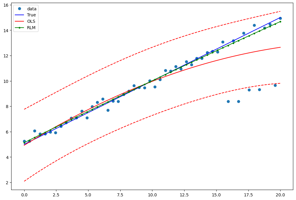
例1: 線形真理値を持つ2次関数
OLS回帰の2次関数が外れ値効果を取り込むことに注意してください。
[8]:
res = sm.OLS(y2, X).fit()
print(res.params)
print(res.bse)
print(res.predict())
[ 5.21792383  0.50415069 -0.01178124]
[0.43595638 0.06730578 0.00595552]
[ 4.92339275  5.17529253  5.42326685  5.66731574  5.90743917  6.14363717
  6.37590971  6.60425681  6.82867847  7.04917468  7.26574545  7.47839077
  7.68711064  7.89190507  8.09277405  8.28971759  8.48273568  8.67182833
  8.85699553  9.03823729  9.2155536   9.38894447  9.55840989  9.72394987
  9.8855644  10.04325348 10.19701712 10.34685531 10.49276806 10.63475536
 10.77281722 10.90695363 11.0371646  11.16345012 11.2858102  11.40424483
 11.51875401 11.62933775 11.73599605 11.8387289  11.9375363  12.03241826
 12.12337477 12.21040584 12.29351146 12.37269164 12.44794637 12.51927566
 12.5866795  12.65015789]
RLMを推定
[9]:
resrlm = sm.RLM(y2, X).fit()
print(resrlm.params)
print(resrlm.bse)
[ 5.15683122e+00  4.88535174e-01 -1.11256925e-03]
[0.12686184 0.01958576 0.00173304]
OLS推定値とロバスト推定値を比較するプロットを描画
[10]:
fig = plt.figure(figsize=(12, 8))
ax = fig.add_subplot(111)
ax.plot(x1, y2, "o", label="data")
ax.plot(x1, y_true2, "b-", label="True")
pred_ols = res.get_prediction()
iv_l = pred_ols.summary_frame()["obs_ci_lower"]
iv_u = pred_ols.summary_frame()["obs_ci_upper"]

ax.plot(x1, res.fittedvalues, "r-", label="OLS")
ax.plot(x1, iv_u, "r--")
ax.plot(x1, iv_l, "r--")
ax.plot(x1, resrlm.fittedvalues, "g.-", label="RLM")
ax.legend(loc="best")
[10]:
<matplotlib.legend.Legend at 0x7ff47df37c10>
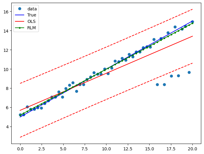
例2: 線形真理値を持つ線形関数
線形項と定数のみを使用する新しいOLSモデルに適合
[11]:
X2 = X[:, [0, 1]]
res2 = sm.OLS(y2, X2).fit()
print(res2.params)
print(res2.bse)
[5.69278005 0.38633826]
[0.37479982 0.03229427]
RLMを推定
[12]:
resrlm2 = sm.RLM(y2, X2).fit()
print(resrlm2.params)
print(resrlm2.bse)
[5.19360532 0.47898089]
[0.10312091 0.00888531]
OLS推定値とロバスト推定値を比較するプロットを描画
[13]:
pred_ols = res2.get_prediction()
iv_l = pred_ols.summary_frame()["obs_ci_lower"]
iv_u = pred_ols.summary_frame()["obs_ci_upper"]

fig, ax = plt.subplots(figsize=(8, 6))
ax.plot(x1, y2, "o", label="data")
ax.plot(x1, y_true2, "b-", label="True")
ax.plot(x1, res2.fittedvalues, "r-", label="OLS")
ax.plot(x1, iv_u, "r--")
ax.plot(x1, iv_l, "r--")
ax.plot(x1, resrlm2.fittedvalues, "g.-", label="RLM")
legend = ax.legend(loc="best")
最終更新日:2024年10月3日