ロバスト線形モデリングのためのM推定量
[1]:
%matplotlib inline
[2]:
from statsmodels.compat import lmap
import numpy as np
from scipy import stats
import matplotlib.pyplot as plt

import statsmodels.api as sm
M推定量は次の関数を最小化します。
ここで、\(\rho\)は残差の対称関数です
\(\rho\)の効果は外れ値の影響を減らすことです
\(s\)は尺度の推定値です。
ロバスト推定値\(\hat{\beta}\)は、反復再重み付け最小二乗アルゴリズムによって計算されます。
使用する重み付け関数にはいくつかの選択肢があります。
[3]:
norms = sm.robust.norms
[4]:
def plot_weights(support, weights_func, xlabels, xticks):
    fig = plt.figure(figsize=(12, 8))
    ax = fig.add_subplot(111)
    ax.plot(support, weights_func(support))
    ax.set_xticks(xticks)
    ax.set_xticklabels(xlabels, fontsize=16)
    ax.set_ylim(-0.1, 1.1)
    return ax
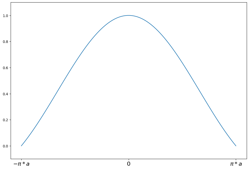
Andrewの波
[5]:
help(norms.AndrewWave.weights)
Help on function weights in module statsmodels.robust.norms:

weights(self, z)
    Andrew's wave weighting function for the IRLS algorithm

    The psi function scaled by z

    Parameters
    ----------
    z : array_like
        1d array

    Returns
    -------
    weights : ndarray
        weights(z) = sin(z/a) / (z/a)     for \|z\| <= a*pi

        weights(z) = 0                    for \|z\| > a*pi
[6]:
a = 1.339
support = np.linspace(-np.pi * a, np.pi * a, 100)
andrew = norms.AndrewWave(a=a)
plot_weights(
    support, andrew.weights, ["$-\pi*a$", "0", "$\pi*a$"], [-np.pi * a, 0, np.pi * a]
)
[6]:
<Axes: >
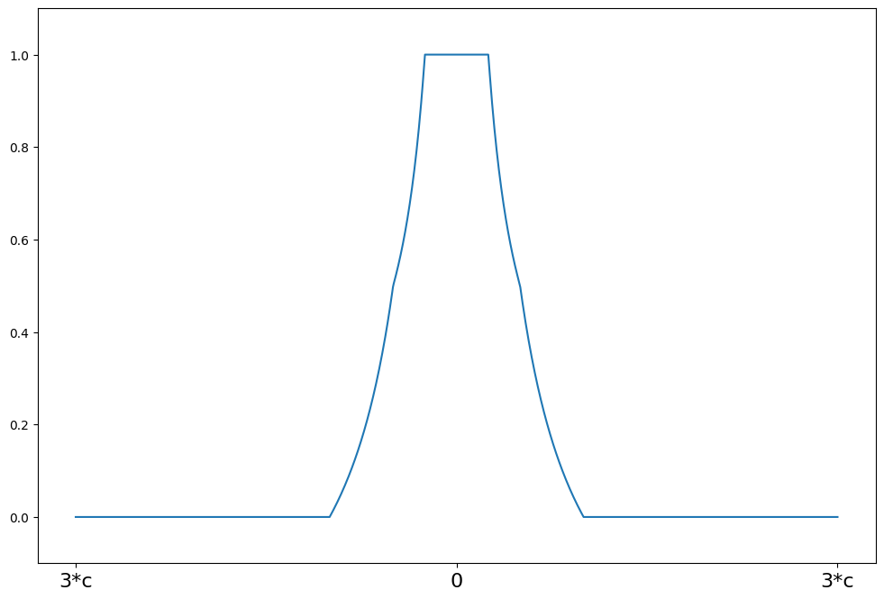
Hampelの17A
[7]:
help(norms.Hampel.weights)
Help on function weights in module statsmodels.robust.norms:

weights(self, z)
    Hampel weighting function for the IRLS algorithm

    The psi function scaled by z

    Parameters
    ----------
    z : array_like
        1d array

    Returns
    -------
    weights : ndarray
        weights(z) = 1                                for \|z\| <= a

        weights(z) = a/\|z\|                          for a < \|z\| <= b

        weights(z) = a*(c - \|z\|)/(\|z\|*(c-b))      for b < \|z\| <= c

        weights(z) = 0                                for \|z\| > c
[8]:
c = 8
support = np.linspace(-3 * c, 3 * c, 1000)
hampel = norms.Hampel(a=2.0, b=4.0, c=c)
plot_weights(support, hampel.weights, ["3*c", "0", "3*c"], [-3 * c, 0, 3 * c])
[8]:
<Axes: >
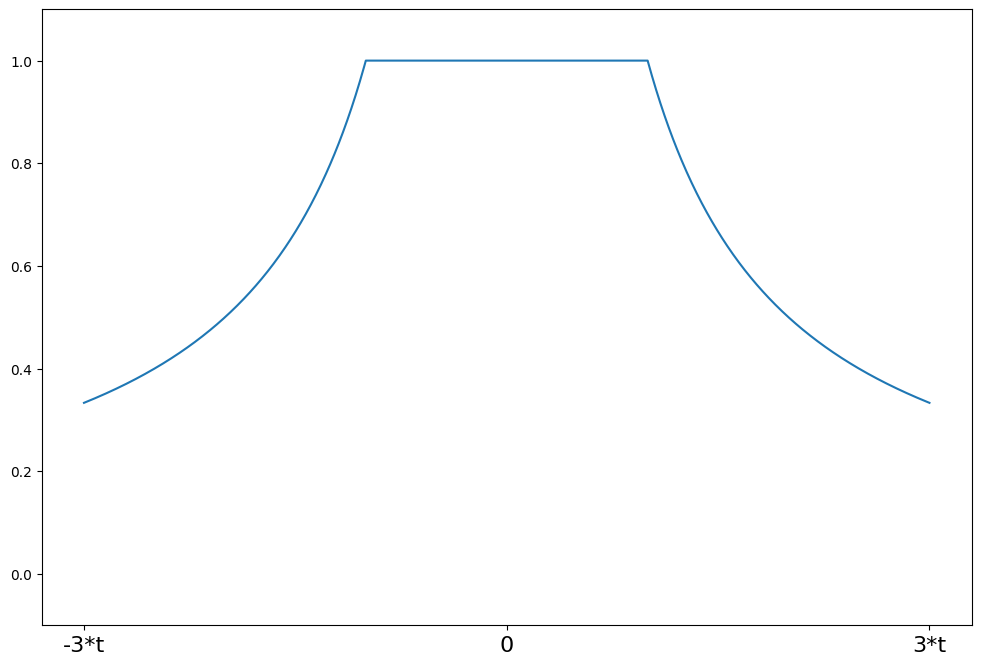
Huberのt
[9]:
help(norms.HuberT.weights)
Help on function weights in module statsmodels.robust.norms:

weights(self, z)
    Huber's t weighting function for the IRLS algorithm

    The psi function scaled by z

    Parameters
    ----------
    z : array_like
        1d array

    Returns
    -------
    weights : ndarray
        weights(z) = 1          for \|z\| <= t

        weights(z) = t/\|z\|      for \|z\| > t
[10]:
t = 1.345
support = np.linspace(-3 * t, 3 * t, 1000)
huber = norms.HuberT(t=t)
plot_weights(support, huber.weights, ["-3*t", "0", "3*t"], [-3 * t, 0, 3 * t])
[10]:
<Axes: >
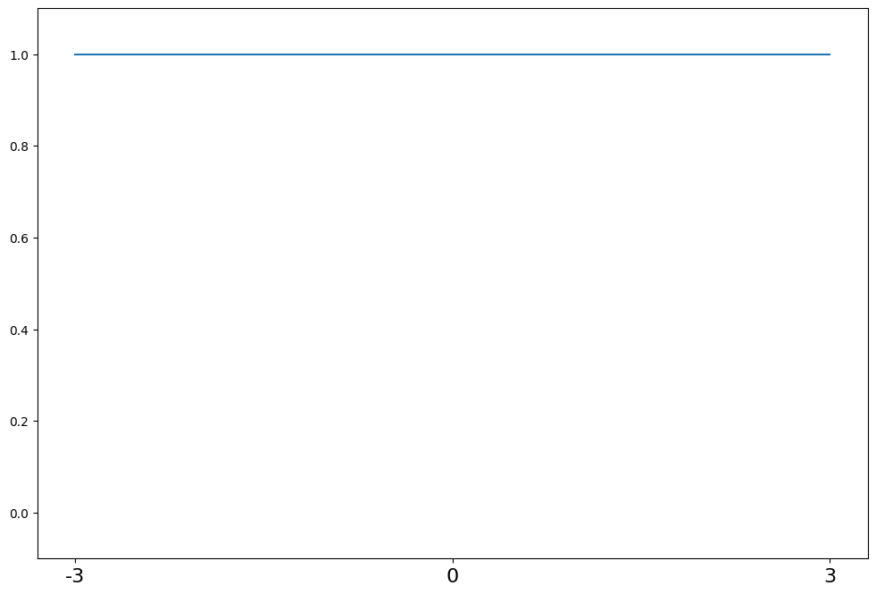
最小二乗法
[11]:
help(norms.LeastSquares.weights)
Help on function weights in module statsmodels.robust.norms:

weights(self, z)
    The least squares estimator weighting function for the IRLS algorithm.

    The psi function scaled by the input z

    Parameters
    ----------
    z : array_like
        1d array

    Returns
    -------
    weights : ndarray
        weights(z) = np.ones(z.shape)
[12]:
support = np.linspace(-3, 3, 1000)
lst_sq = norms.LeastSquares()
plot_weights(support, lst_sq.weights, ["-3", "0", "3"], [-3, 0, 3])
[12]:
<Axes: >
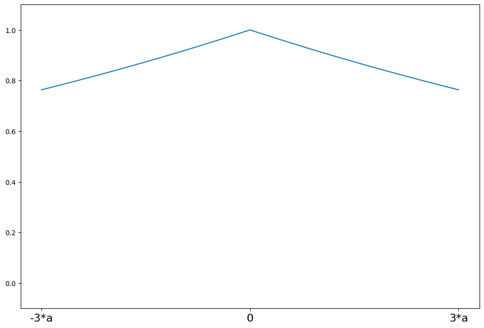
RamsayのEa
[13]:
help(norms.RamsayE.weights)
Help on function weights in module statsmodels.robust.norms:

weights(self, z)
    Ramsay's Ea weighting function for the IRLS algorithm

    The psi function scaled by z

    Parameters
    ----------
    z : array_like
        1d array

    Returns
    -------
    weights : ndarray
        weights(z) = exp(-a*\|z\|)
[14]:
a = 0.3
support = np.linspace(-3 * a, 3 * a, 1000)
ramsay = norms.RamsayE(a=a)
plot_weights(support, ramsay.weights, ["-3*a", "0", "3*a"], [-3 * a, 0, 3 * a])
[14]:
<Axes: >
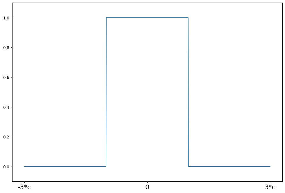
トリム平均
[15]:
help(norms.TrimmedMean.weights)
Help on function weights in module statsmodels.robust.norms:

weights(self, z)
    Least trimmed mean weighting function for the IRLS algorithm

    The psi function scaled by z

    Parameters
    ----------
    z : array_like
        1d array

    Returns
    -------
    weights : ndarray
        weights(z) = 1             for \|z\| <= c

        weights(z) = 0             for \|z\| > c
[16]:
c = 2
support = np.linspace(-3 * c, 3 * c, 1000)
trimmed = norms.TrimmedMean(c=c)
plot_weights(support, trimmed.weights, ["-3*c", "0", "3*c"], [-3 * c, 0, 3 * c])
[16]:
<Axes: >
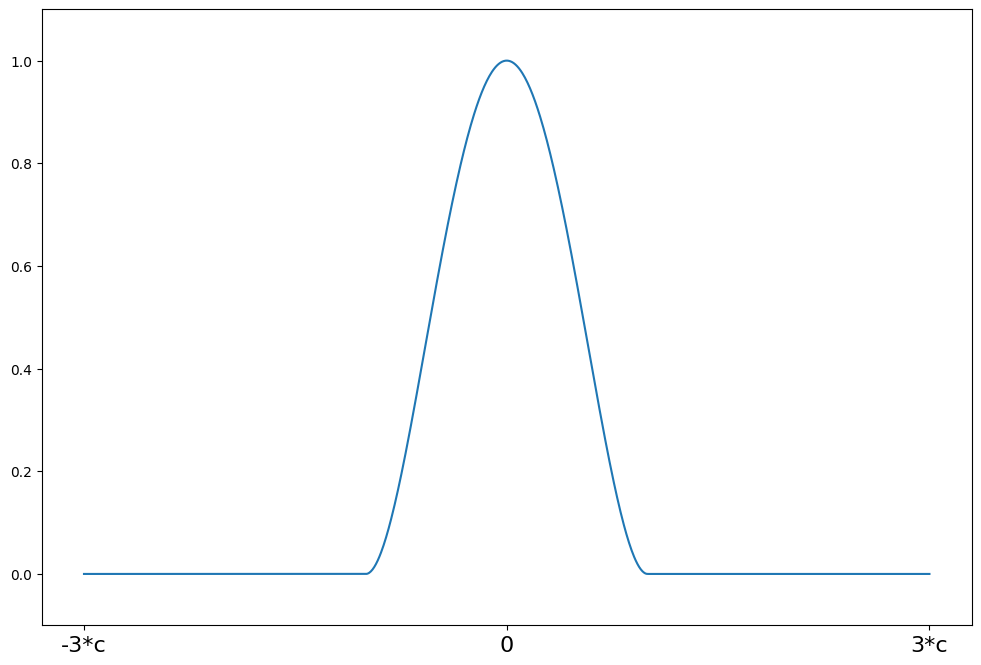
TukeyのBiweight
[17]:
help(norms.TukeyBiweight.weights)
Help on function weights in module statsmodels.robust.norms:

weights(self, z)
    Tukey's biweight weighting function for the IRLS algorithm

    The psi function scaled by z

    Parameters
    ----------
    z : array_like
        1d array

    Returns
    -------
    weights : ndarray
        psi(z) = (1 - (z/c)**2)**2          for \|z\| <= R

        psi(z) = 0                          for \|z\| > R
[18]:
c = 4.685
support = np.linspace(-3 * c, 3 * c, 1000)
tukey = norms.TukeyBiweight(c=c)
plot_weights(support, tukey.weights, ["-3*c", "0", "3*c"], [-3 * c, 0, 3 * c])
[18]:
<Axes: >
尺度推定量
位置のロバスト推定
[19]:
x = np.array([1, 2, 3, 4, 500])
平均は位置のロバスト推定量ではありません
[20]:
x.mean()
[20]:
np.float64(102.0)
一方、中央値はブレークダウン点が50%のロバスト推定量です。
[21]:
np.median(x)
[21]:
np.float64(3.0)
尺度についても同様です
標準偏差はロバストではありません
[22]:
x.std()
[22]:
np.float64(199.00251254695254)
中央絶対偏差
標準化された中央絶対偏差は、\(\hat{\sigma}\)の一致推定量です
ここで、\(K\)は分布に依存します。たとえば、正規分布の場合、
[23]:
stats.norm.ppf(0.75)
[23]:
np.float64(0.6744897501960817)
[24]:
print(x)
[ 1 2 3 4 500]
[25]:
sm.robust.scale.mad(x)
[25]:
np.float64(1.482602218505602)
[26]:
np.array([1, 2, 3, 4, 5.0]).std()
[26]:
np.float64(1.4142135623730951)
尺度の別のロバスト推定量は四分位範囲(IQR)です。
ここで、\(\hat{X}_{p}\)はサンプルのp番目の分位数であり、\(K\)は分布に依存します。
標準化されたIQRは、\(K \cdot \text{IQR}\)で与えられ、
は、正規データに対する標準偏差の一致推定量です。
[27]:
sm.robust.scale.iqr(x)
[27]:
array(1.48260222)
IQRは、完全に崩壊する前に25%の外れ値観測に耐えることができ、MADは50%の外れ値観測に耐えることができるという意味で、MADよりもロバスト性が低くなります。ただし、IQRは非対称分布により適しています。
尺度の別のロバスト推定量は、Rousseeuw&Croux(1993)の「中央絶対偏差の代替」で導入された\(Q_n\)推定量です。次に、\(Q_n\)推定量は次のように与えられます。
ここで、\(h\approx (1/4){{n}\choose{2}}\)であり、\(K\)は所与の定数です。言葉で言えば、\(Q_n\)推定量は、データの絶対差の正規化された\(h\)番目の順序統計量です。正規化定数\(K\)は通常、正規データの場合に推定量を標準偏差と一致させるために、2.219144として選択されます。\(Q_n\)推定量は50%のブレークダウン点と正規分布で82%の漸近効率を持っており、MADの37%の効率よりもはるかに高くなっています。
[28]:
sm.robust.scale.qn_scale(x)
[28]:
2.219144465985076
ロバスト線形モデルのデフォルトはMADです
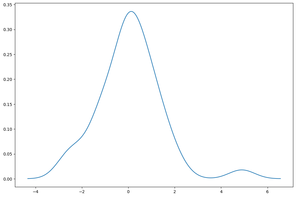
別の一般的な選択肢はHuberの提案2です
[29]:
np.random.seed(12345)
fat_tails = stats.t(6).rvs(40)
[30]:
kde = sm.nonparametric.KDEUnivariate(fat_tails)
kde.fit()
fig = plt.figure(figsize=(12, 8))
ax = fig.add_subplot(111)
ax.plot(kde.support, kde.density)
[30]:
[<matplotlib.lines.Line2D at 0x7f1eaab6baf0>]
[31]:
print(fat_tails.mean(), fat_tails.std())
0.0688231044810875 1.3471633229698652
[32]:
print(stats.norm.fit(fat_tails))
(np.float64(0.0688231044810875), np.float64(1.3471633229698652))
[33]:
print(stats.t.fit(fat_tails, f0=6))
(6, np.float64(0.03900835312789366), np.float64(1.0563837144431252))
[34]:
huber = sm.robust.scale.Huber()
loc, scale = huber(fat_tails)
print(loc, scale)
0.04048984333271795 1.1557140047569665
[35]:
sm.robust.mad(fat_tails)
[35]:
np.float64(1.115335001165415)
[36]:
sm.robust.mad(fat_tails, c=stats.t(6).ppf(0.75))
[36]:
np.float64(1.0483916565928972)
[37]:
sm.robust.scale.mad(fat_tails)
[37]:
np.float64(1.115335001165415)
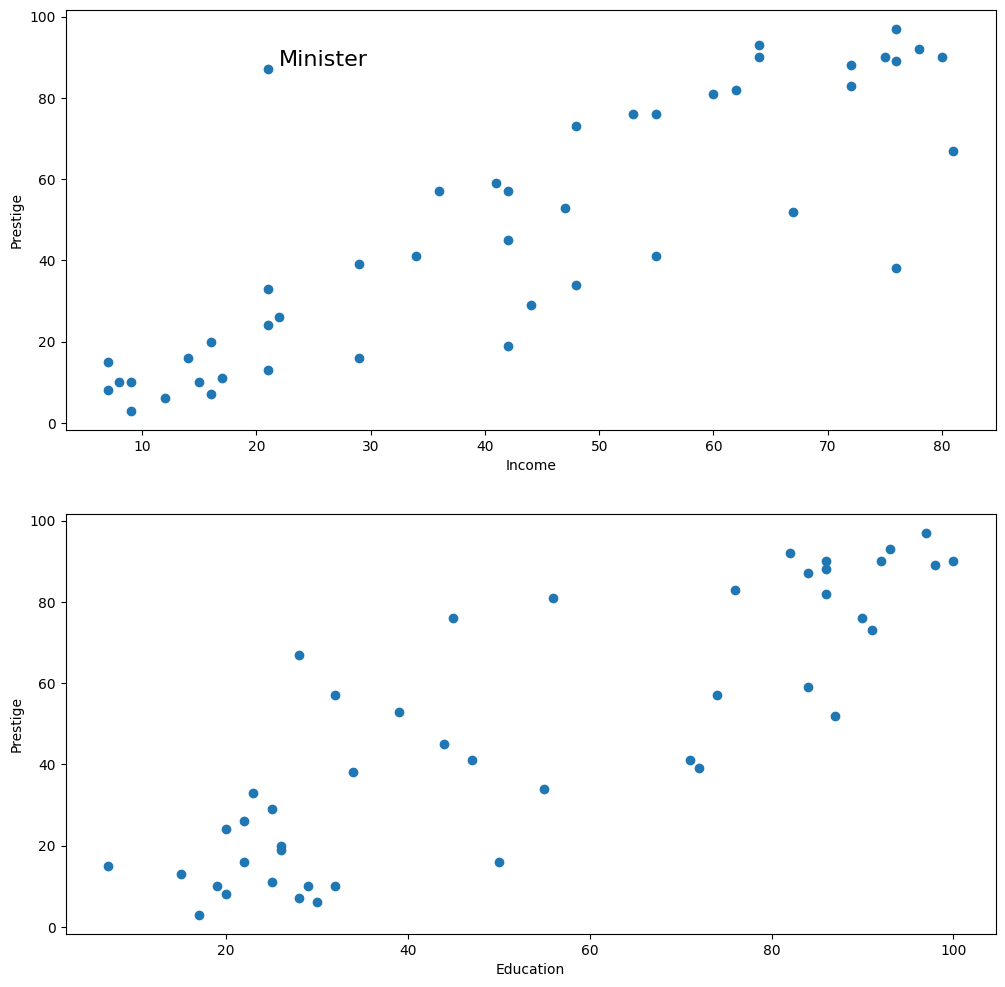
ダンカンの職業的威信データ - 外れ値に対するM推定
[38]:
from statsmodels.graphics.api import abline_plot
from statsmodels.formula.api import ols, rlm
[39]:
prestige = sm.datasets.get_rdataset("Duncan", "carData", cache=True).data
[40]:
print(prestige.head(10))
            type  income  education  prestige
rownames
accountant  prof      62         86        82
pilot       prof      72         76        83
architect   prof      75         92        90
author      prof      55         90        76
chemist     prof      64         86        90
minister    prof      21         84        87
professor   prof      64         93        93
dentist     prof      80        100        90
reporter      wc      67         87        52
engineer    prof      72         86        88
[41]:
fig = plt.figure(figsize=(12, 12))
ax1 = fig.add_subplot(211, xlabel="Income", ylabel="Prestige")
ax1.scatter(prestige.income, prestige.prestige)
xy_outlier = prestige.loc["minister", ["income", "prestige"]]
ax1.annotate("Minister", xy_outlier, xy_outlier + 1, fontsize=16)
ax2 = fig.add_subplot(212, xlabel="Education", ylabel="Prestige")
ax2.scatter(prestige.education, prestige.prestige)
[41]:
<matplotlib.collections.PathCollection at 0x7f1eaaa78670>
[42]:
ols_model = ols("prestige ~ income + education", prestige).fit()
print(ols_model.summary())
                            OLS Regression Results
==============================================================================
Dep. Variable:               prestige   R-squared:                       0.828
Model:                            OLS   Adj. R-squared:                  0.820
Method:                 Least Squares   F-statistic:                     101.2
Date:                Thu, 03 Oct 2024   Prob (F-statistic):           8.65e-17
Time:                        15:58:23   Log-Likelihood:                -178.98
No. Observations:                  45   AIC:                             364.0
Df Residuals:                      42   BIC:                             369.4
Df Model:                           2
Covariance Type:            nonrobust
==============================================================================
                 coef    std err          t      P>|t|      [0.025      0.975]
------------------------------------------------------------------------------
Intercept     -6.0647      4.272     -1.420      0.163     -14.686       2.556
income         0.5987      0.120      5.003      0.000       0.357       0.840
education      0.5458      0.098      5.555      0.000       0.348       0.744
==============================================================================
Omnibus:                        1.279   Durbin-Watson:                   1.458
Prob(Omnibus):                  0.528   Jarque-Bera (JB):                0.520
Skew:                           0.155   Prob(JB):                        0.771
Kurtosis:                       3.426   Cond. No.                         163.
==============================================================================

Notes:
[1] Standard Errors assume that the covariance matrix of the errors is correctly specified.
[43]:
infl = ols_model.get_influence()
student = infl.summary_frame()["student_resid"]
print(student)
rownames
accountant            0.303900
pilot                 0.340920
architect             0.072256
author                0.000711
chemist               0.826578
minister              3.134519
professor             0.768277
dentist              -0.498082
reporter             -2.397022
engineer              0.306225
undertaker           -0.187339
lawyer               -0.303082
physician             0.355687
welfare.worker       -0.411406
teacher               0.050510
conductor            -1.704032
contractor            2.043805
factory.owner         1.602429
store.manager         0.142425
banker                0.508388
bookkeeper           -0.902388
mail.carrier         -1.433249
insurance.agent      -1.930919
store.clerk          -1.760491
carpenter             1.068858
electrician           0.731949
RR.engineer           0.808922
machinist             1.887047
auto.repairman        0.522735
plumber              -0.377954
gas.stn.attendant    -0.666596
coal.miner            1.018527
streetcar.motorman   -1.104485
taxi.driver           0.023322
truck.driver         -0.129227
machine.operator      0.499922
barber                0.173805
bartender            -0.902422
shoe.shiner          -0.429357
cook                  0.127207
soda.clerk           -0.883095
watchman             -0.513502
janitor              -0.079890
policeman             0.078847
waiter               -0.475972
Name: student_resid, dtype: float64
[44]:
print(student.loc[np.abs(student) > 2])
rownames
minister      3.134519
reporter     -2.397022
contractor    2.043805
Name: student_resid, dtype: float64
[45]:
print(infl.summary_frame().loc["minister"])
dfb_Intercept      0.144937
dfb_income        -1.220939
dfb_education      1.263019
cooks_d            0.566380
standard_resid     2.849416
hat_diag           0.173058
dffits_internal    1.303510
student_resid      3.134519
dffits             1.433935
Name: minister, dtype: float64
[46]:
sidak = ols_model.outlier_test("sidak")
sidak.sort_values("unadj_p", inplace=True)
print(sidak)
                    student_resid   unadj_p  sidak(p)
minister                 3.134519  0.003177  0.133421
reporter                -2.397022  0.021170  0.618213
contractor               2.043805  0.047433  0.887721
insurance.agent         -1.930919  0.060428  0.939485
machinist                1.887047  0.066248  0.954247
store.clerk             -1.760491  0.085783  0.982331
conductor               -1.704032  0.095944  0.989315
factory.owner            1.602429  0.116738  0.996250
mail.carrier            -1.433249  0.159369  0.999595
streetcar.motorman      -1.104485  0.275823  1.000000
carpenter                1.068858  0.291386  1.000000
coal.miner               1.018527  0.314400  1.000000
bartender               -0.902422  0.372104  1.000000
bookkeeper              -0.902388  0.372122  1.000000
soda.clerk              -0.883095  0.382334  1.000000
chemist                  0.826578  0.413261  1.000000
RR.engineer              0.808922  0.423229  1.000000
professor                0.768277  0.446725  1.000000
electrician              0.731949  0.468363  1.000000
gas.stn.attendant       -0.666596  0.508764  1.000000
auto.repairman           0.522735  0.603972  1.000000
watchman                -0.513502  0.610357  1.000000
banker                   0.508388  0.613906  1.000000
machine.operator         0.499922  0.619802  1.000000
dentist                 -0.498082  0.621088  1.000000
waiter                  -0.475972  0.636621  1.000000
shoe.shiner             -0.429357  0.669912  1.000000
welfare.worker          -0.411406  0.682918  1.000000
plumber                 -0.377954  0.707414  1.000000
physician                0.355687  0.723898  1.000000
pilot                    0.340920  0.734905  1.000000
engineer                 0.306225  0.760983  1.000000
accountant               0.303900  0.762741  1.000000
lawyer                  -0.303082  0.763360  1.000000
undertaker              -0.187339  0.852319  1.000000
barber                   0.173805  0.862874  1.000000
store.manager            0.142425  0.887442  1.000000
truck.driver            -0.129227  0.897810  1.000000
cook                     0.127207  0.899399  1.000000
janitor                 -0.079890  0.936713  1.000000
policeman                0.078847  0.937538  1.000000
architect                0.072256  0.942750  1.000000
teacher                  0.050510  0.959961  1.000000
taxi.driver              0.023322  0.981507  1.000000
author                   0.000711  0.999436  1.000000
[47]:
fdr = ols_model.outlier_test("fdr_bh")
fdr.sort_values("unadj_p", inplace=True)
print(fdr)
                    student_resid   unadj_p  fdr_bh(p)
minister                 3.134519  0.003177   0.142974
reporter                -2.397022  0.021170   0.476332
contractor               2.043805  0.047433   0.596233
insurance.agent         -1.930919  0.060428   0.596233
machinist                1.887047  0.066248   0.596233
store.clerk             -1.760491  0.085783   0.616782
conductor               -1.704032  0.095944   0.616782
factory.owner            1.602429  0.116738   0.656653
mail.carrier            -1.433249  0.159369   0.796844
streetcar.motorman      -1.104485  0.275823   0.999436
carpenter                1.068858  0.291386   0.999436
coal.miner               1.018527  0.314400   0.999436
bartender               -0.902422  0.372104   0.999436
bookkeeper              -0.902388  0.372122   0.999436
soda.clerk              -0.883095  0.382334   0.999436
chemist                  0.826578  0.413261   0.999436
RR.engineer              0.808922  0.423229   0.999436
professor                0.768277  0.446725   0.999436
electrician              0.731949  0.468363   0.999436
gas.stn.attendant       -0.666596  0.508764   0.999436
auto.repairman           0.522735  0.603972   0.999436
watchman                -0.513502  0.610357   0.999436
banker                   0.508388  0.613906   0.999436
machine.operator         0.499922  0.619802   0.999436
dentist                 -0.498082  0.621088   0.999436
waiter                  -0.475972  0.636621   0.999436
shoe.shiner             -0.429357  0.669912   0.999436
welfare.worker          -0.411406  0.682918   0.999436
plumber                 -0.377954  0.707414   0.999436
physician                0.355687  0.723898   0.999436
pilot                    0.340920  0.734905   0.999436
engineer                 0.306225  0.760983   0.999436
accountant               0.303900  0.762741   0.999436
lawyer                  -0.303082  0.763360   0.999436
undertaker              -0.187339  0.852319   0.999436
barber                   0.173805  0.862874   0.999436
store.manager            0.142425  0.887442   0.999436
truck.driver            -0.129227  0.897810   0.999436
cook                     0.127207  0.899399   0.999436
janitor                 -0.079890  0.936713   0.999436
policeman                0.078847  0.937538   0.999436
architect                0.072256  0.942750   0.999436
teacher                  0.050510  0.959961   0.999436
taxi.driver              0.023322  0.981507   0.999436
author                   0.000711  0.999436   0.999436
[48]:
rlm_model = rlm("prestige ~ income + education", prestige).fit()
print(rlm_model.summary())
                    Robust linear Model Regression Results
==============================================================================
Dep. Variable:               prestige   No. Observations:                   45
Model:                            RLM   Df Residuals:                       42
Method:                          IRLS   Df Model:                            2
Norm:                          HuberT
Scale Est.:                       mad
Cov Type:                          H1
Date:                Thu, 03 Oct 2024
Time:                        15:58:23
No. Iterations:                    18
==============================================================================
                 coef    std err          z      P>|z|      [0.025      0.975]
------------------------------------------------------------------------------
Intercept     -7.1107      3.879     -1.833      0.067     -14.713       0.492
income         0.7015      0.109      6.456      0.000       0.489       0.914
education      0.4854      0.089      5.441      0.000       0.311       0.660
==============================================================================

If the model instance has been used for another fit with different fit parameters, then the fit options might not be the correct ones anymore .
[49]:
print(rlm_model.weights)
rownames
accountant            1.000000
pilot                 1.000000
architect             1.000000
author                1.000000
chemist               1.000000
minister              0.344596
professor             1.000000
dentist               1.000000
reporter              0.441669
engineer              1.000000
undertaker            1.000000
lawyer                1.000000
physician             1.000000
welfare.worker        1.000000
teacher               1.000000
conductor             0.538445
contractor            0.552262
factory.owner         0.706169
store.manager         1.000000
banker                1.000000
bookkeeper            1.000000
mail.carrier          0.690764
insurance.agent       0.533499
store.clerk           0.618656
carpenter             0.935848
electrician           1.000000
RR.engineer           1.000000
machinist             0.570360
auto.repairman        1.000000
plumber               1.000000
gas.stn.attendant     1.000000
coal.miner            0.963821
streetcar.motorman    0.832870
taxi.driver           1.000000
truck.driver          1.000000
machine.operator      1.000000
barber                1.000000
bartender             1.000000
shoe.shiner           1.000000
cook                  1.000000
soda.clerk            1.000000
watchman              1.000000
janitor               1.000000
policeman             1.000000
waiter                1.000000
dtype: float64
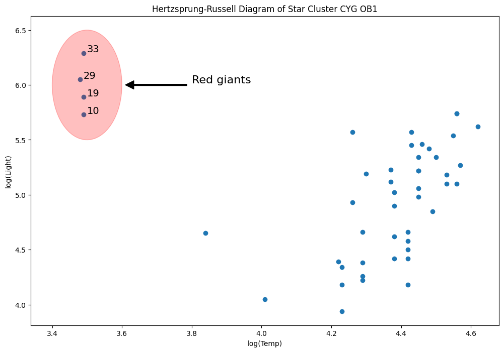
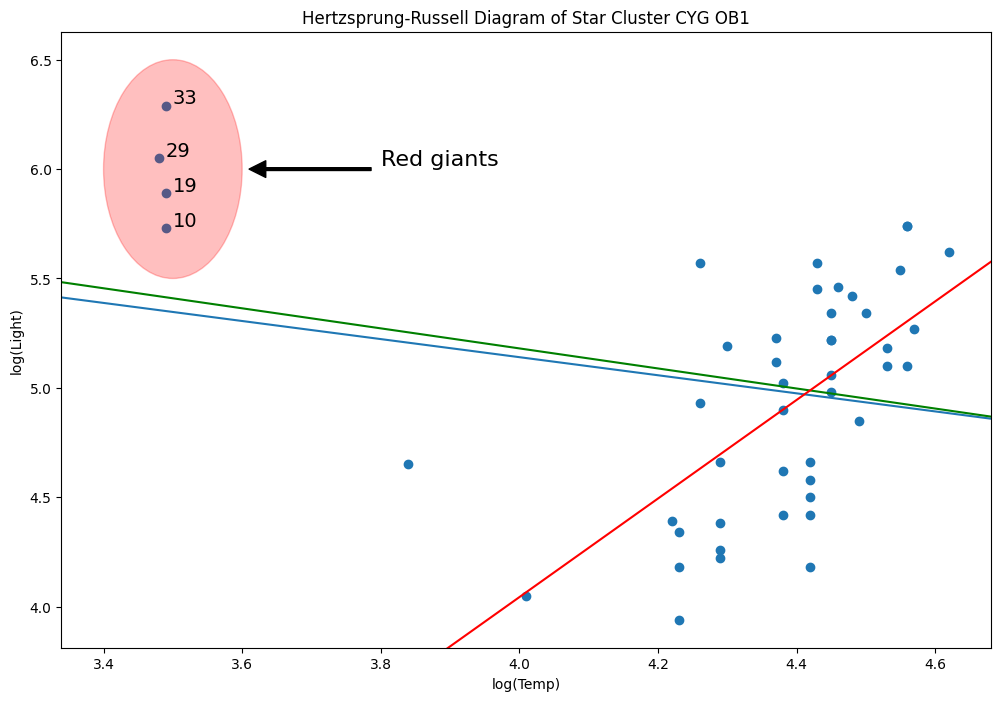
星団CYG 0B1のヘルツシュプルング・ラッセル図 - レバレッジ点
データは、はくちょう座の方向にある47個の星の光度と温度に関するものです。
[50]:
dta = sm.datasets.get_rdataset("starsCYG", "robustbase", cache=True).data
[51]:
from matplotlib.patches import Ellipse

fig = plt.figure(figsize=(12, 8))
ax = fig.add_subplot(
    111,
    xlabel="log(Temp)",
    ylabel="log(Light)",
    title="Hertzsprung-Russell Diagram of Star Cluster CYG OB1",
)
ax.scatter(*dta.values.T)
# highlight outliers
e = Ellipse((3.5, 6), 0.2, 1, alpha=0.25, color="r")
ax.add_patch(e)
ax.annotate(
    "Red giants",
    xy=(3.6, 6),
    xytext=(3.8, 6),
    arrowprops=dict(facecolor="black", shrink=0.05, width=2),
    horizontalalignment="left",
    verticalalignment="bottom",
    clip_on=True,  # clip to the axes bounding box
    fontsize=16,
)
# annotate these with their index
for i, row in dta.loc[dta["log.Te"] < 3.8].iterrows():
    ax.annotate(i, row, row + 0.01, fontsize=14)
xlim, ylim = ax.get_xlim(), ax.get_ylim()
[52]:
from IPython.display import Image

Image(filename="star_diagram.png")
[52]:

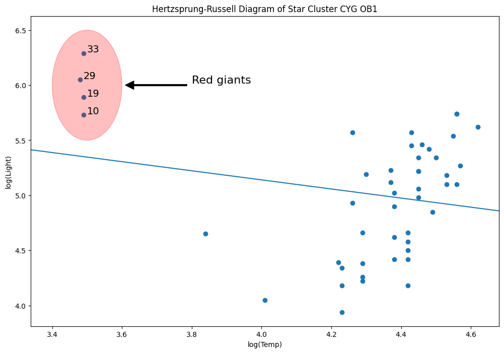
[53]:
y = dta["log.light"]
X = sm.add_constant(dta["log.Te"], prepend=True)
ols_model = sm.OLS(y, X).fit()
abline_plot(model_results=ols_model, ax=ax)
[53]:
[54]:
rlm_mod = sm.RLM(y, X, sm.robust.norms.TrimmedMean(0.5)).fit()
abline_plot(model_results=rlm_mod, ax=ax, color="red")
[54]:
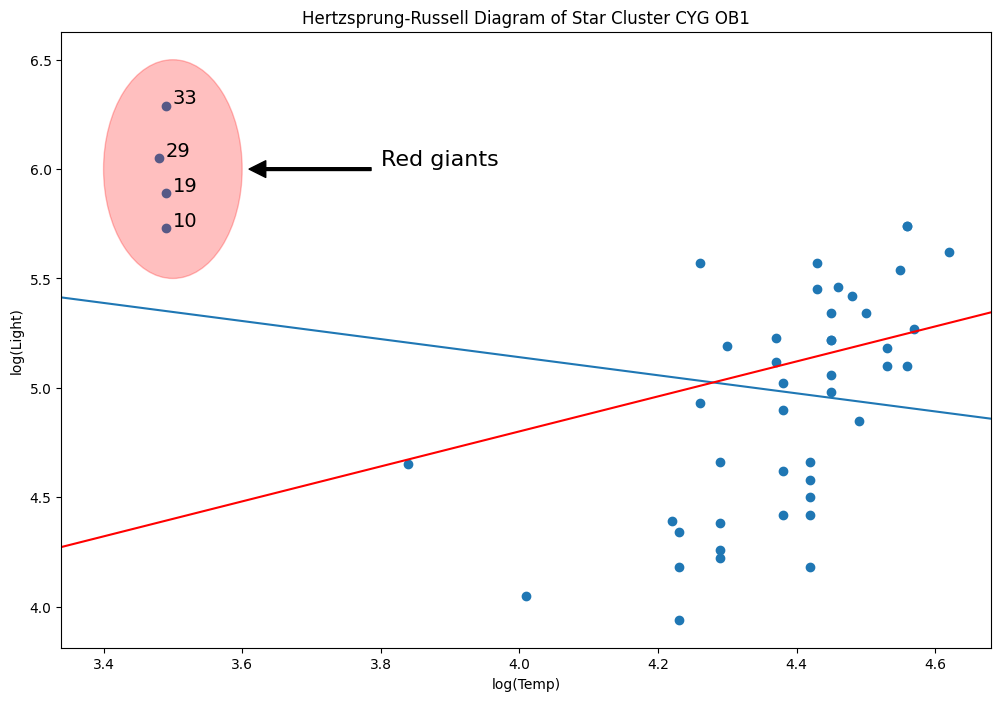
なぜ? M推定量はレバレッジ点に対してロバストではないからです。
[55]:
infl = ols_model.get_influence()
[56]:
h_bar = 2 * (ols_model.df_model + 1) / ols_model.nobs
hat_diag = infl.summary_frame()["hat_diag"]
hat_diag.loc[hat_diag > h_bar]
[56]:
10    0.194103
19    0.194103
29    0.198344
33    0.194103
Name: hat_diag, dtype: float64
[57]:
sidak2 = ols_model.outlier_test("sidak")
sidak2.sort_values("unadj_p", inplace=True)
print(sidak2)
    student_resid   unadj_p  sidak(p)
16      -2.049393  0.046415  0.892872
13      -2.035329  0.047868  0.900286
33       1.905847  0.063216  0.953543
18      -1.575505  0.122304  0.997826
3        1.522185  0.135118  0.998911
1        1.522185  0.135118  0.998911
21      -1.450418  0.154034  0.999615
17      -1.426675  0.160731  0.999735
29       1.388520  0.171969  0.999859
14      -1.374733  0.176175  0.999889
35       1.346543  0.185023  0.999933
34      -1.272159  0.209999  0.999985
28      -1.186946  0.241618  0.999998
20      -1.150621  0.256103  0.999999
44       1.134779  0.262612  0.999999
39       1.091886  0.280826  1.000000
19       1.064878  0.292740  1.000000
6       -1.026873  0.310093  1.000000
30      -1.009096  0.318446  1.000000
22      -0.979768  0.332557  1.000000
8        0.961218  0.341695  1.000000
5        0.913802  0.365801  1.000000
11       0.871997  0.387943  1.000000
12       0.856685  0.396261  1.000000
46      -0.833923  0.408829  1.000000
10       0.743920  0.460879  1.000000
42       0.727179  0.470968  1.000000
15      -0.689258  0.494280  1.000000
43       0.688272  0.494895  1.000000
7        0.655712  0.515424  1.000000
40      -0.646396  0.521381  1.000000
26      -0.640978  0.524862  1.000000
25      -0.545561  0.588123  1.000000
37       0.472819  0.638680  1.000000
32       0.472819  0.638680  1.000000
38       0.462187  0.646225  1.000000
0        0.430686  0.668799  1.000000
31       0.341726  0.734184  1.000000
36       0.318911  0.751303  1.000000
4        0.307890  0.759619  1.000000
9        0.235114  0.815211  1.000000
41       0.187732  0.851950  1.000000
2       -0.182093  0.856346  1.000000
23      -0.156014  0.876736  1.000000
27      -0.147406  0.883485  1.000000
24       0.065195  0.948314  1.000000
45       0.045675  0.963776  1.000000
[58]:
fdr2 = ols_model.outlier_test("fdr_bh")
fdr2.sort_values("unadj_p", inplace=True)
print(fdr2)
    student_resid   unadj_p  fdr_bh(p)
16      -2.049393  0.046415   0.764747
13      -2.035329  0.047868   0.764747
33       1.905847  0.063216   0.764747
18      -1.575505  0.122304   0.764747
3        1.522185  0.135118   0.764747
1        1.522185  0.135118   0.764747
21      -1.450418  0.154034   0.764747
17      -1.426675  0.160731   0.764747
29       1.388520  0.171969   0.764747
14      -1.374733  0.176175   0.764747
35       1.346543  0.185023   0.764747
34      -1.272159  0.209999   0.764747
28      -1.186946  0.241618   0.764747
20      -1.150621  0.256103   0.764747
44       1.134779  0.262612   0.764747
39       1.091886  0.280826   0.764747
19       1.064878  0.292740   0.764747
6       -1.026873  0.310093   0.764747
30      -1.009096  0.318446   0.764747
22      -0.979768  0.332557   0.764747
8        0.961218  0.341695   0.764747
5        0.913802  0.365801   0.768599
11       0.871997  0.387943   0.768599
12       0.856685  0.396261   0.768599
46      -0.833923  0.408829   0.768599
10       0.743920  0.460879   0.770890
42       0.727179  0.470968   0.770890
15      -0.689258  0.494280   0.770890
43       0.688272  0.494895   0.770890
7        0.655712  0.515424   0.770890
40      -0.646396  0.521381   0.770890
26      -0.640978  0.524862   0.770890
25      -0.545561  0.588123   0.837630
37       0.472819  0.638680   0.843682
32       0.472819  0.638680   0.843682
38       0.462187  0.646225   0.843682
0        0.430686  0.668799   0.849556
31       0.341726  0.734184   0.892552
36       0.318911  0.751303   0.892552
4        0.307890  0.759619   0.892552
9        0.235114  0.815211   0.922751
41       0.187732  0.851950   0.922751
2       -0.182093  0.856346   0.922751
23      -0.156014  0.876736   0.922751
27      -0.147406  0.883485   0.922751
24       0.065195  0.948314   0.963776
45       0.045675  0.963776   0.963776
その行を削除しましょう
[59]:
l = ax.lines[-1]
l.remove()
del l
[60]:
weights = np.ones(len(X))
weights[X[X["log.Te"] < 3.8].index.values - 1] = 0
wls_model = sm.WLS(y, X, weights=weights).fit()
abline_plot(model_results=wls_model, ax=ax, color="green")
[60]:

MM推定量はこのタイプの問題に適していますが、残念ながら、まだこれらを使用できません。
それに取り組んでいますが、ノートブックでRセルマジックを見る良い機会になります。
[61]:
yy = y.values[:, None]
xx = X["log.Te"].values[:, None]
注:このノートブックのRコードと結果は、ドキュメントを構築するためにRが不要になるようにmarkdownに変換されました。ノートブックのRの結果は、R 3.5.1とrobustbase 0.93を使用して計算されました。
%load_ext rpy2.ipython

%R library(robustbase)
%Rpush yy xx
%R mod <- lmrob(yy ~ xx);
%R params <- mod$coefficients;
%Rpull params
%R print(mod)
Call:
lmrob(formula = yy ~ xx)
 \--> method = "MM"
Coefficients:
(Intercept)           xx
     -4.969        2.253
[62]:
params = [-4.969387980288108, 2.2531613477892365]  # Computed using R
print(params[0], params[1])
-4.969387980288108 2.2531613477892365
[63]:
abline_plot(intercept=params[0], slope=params[1], ax=ax, color="red")
[63]:
演習:M推定量のブレークダウン点
[64]:
np.random.seed(12345)
nobs = 200
beta_true = np.array([3, 1, 2.5, 3, -4])
X = np.random.uniform(-20, 20, size=(nobs, len(beta_true) - 1))
# stack a constant in front
X = sm.add_constant(X, prepend=True)  # np.c_[np.ones(nobs), X]
mc_iter = 500
contaminate = 0.25  # percentage of response variables to contaminate
[65]:
all_betas = []
for i in range(mc_iter):
    y = np.dot(X, beta_true) + np.random.normal(size=200)
    random_idx = np.random.randint(0, nobs, size=int(contaminate * nobs))
    y[random_idx] = np.random.uniform(-750, 750)
    beta_hat = sm.RLM(y, X).fit().params
    all_betas.append(beta_hat)
[66]:
all_betas = np.asarray(all_betas)
se_loss = lambda x: np.linalg.norm(x, ord=2) ** 2
se_beta = lmap(se_loss, all_betas - beta_true)
二乗誤差損失
[67]:
np.array(se_beta).mean()
[67]:
np.float64(0.44502948730683384)
[68]:
all_betas.mean(0)
[68]:
array([ 2.99711706, 0.99898147, 2.49909344, 2.99712918, -3.99626521])
[69]:
beta_true
[69]:
array([ 3. , 1. , 2.5, 3. , -4. ])
[70]:
se_loss(all_betas.mean(0) - beta_true)
[70]:
np.float64(3.236091328690045e-05)