回帰プロット
[1]:
%matplotlib inline
[2]:
from statsmodels.compat import lzip
import numpy as np
import matplotlib.pyplot as plt
import statsmodels.api as sm
from statsmodels.formula.api import ols

plt.rc("figure", figsize=(16, 8))
plt.rc("font", size=14)
ダンカンの職業威信データセット
データのロード
Rdatasetsパッケージで利用可能な任意のRデータセットをロードするためのユーティリティ関数を使用できます。
[3]:
prestige = sm.datasets.get_rdataset("Duncan", "carData", cache=True).data
[4]:
prestige.head()
[4]:
| type | income | education | prestige | |
|---|---|---|---|---|
| rownames | ||||
| accountant | prof | 62 | 86 | 82 |
| pilot | prof | 72 | 76 | 83 |
| architect | prof | 75 | 92 | 90 |
| author | prof | 55 | 90 | 76 |
| chemist | prof | 64 | 86 | 90 |
[5]:
prestige_model = ols("prestige ~ income + education", data=prestige).fit()
[6]:
print(prestige_model.summary())
                            OLS Regression Results
==============================================================================
Dep. Variable:               prestige   R-squared:                       0.828
Model:                            OLS   Adj. R-squared:                  0.820
Method:                 Least Squares   F-statistic:                     101.2
Date:                Thu, 03 Oct 2024   Prob (F-statistic):           8.65e-17
Time:                        15:58:25   Log-Likelihood:                -178.98
No. Observations:                  45   AIC:                             364.0
Df Residuals:                      42   BIC:                             369.4
Df Model:                           2
Covariance Type:            nonrobust
==============================================================================
                 coef    std err          t      P>|t|      [0.025      0.975]
------------------------------------------------------------------------------
Intercept     -6.0647      4.272     -1.420      0.163     -14.686       2.556
income         0.5987      0.120      5.003      0.000       0.357       0.840
education      0.5458      0.098      5.555      0.000       0.348       0.744
==============================================================================
Omnibus:                        1.279   Durbin-Watson:                   1.458
Prob(Omnibus):                  0.528   Jarque-Bera (JB):                0.520
Skew:                           0.155   Prob(JB):                        0.771
Kurtosis:                       3.426   Cond. No.                         163.
==============================================================================

Notes:
[1] Standard Errors assume that the covariance matrix of the errors is correctly specified.
影響度プロット
影響度プロットは、ハット行列で測定される各観測値のレバレッジに対する(外部)スチューデント化残差を示します。
外部スチューデント化残差は、標準偏差でスケーリングされた残差であり、ここでは
ここで、
\(n\) は観測値の数であり、\(p\) は回帰変数の数です。\(h_{ii}\) はハット行列の \(i\) 番目の対角要素です。
各点の影響は、キーワード引数criterionによって可視化できます。オプションは、影響の2つの尺度であるCookの距離とDFFITSです。
[7]:
fig = sm.graphics.influence_plot(prestige_model, criterion="cooks")
fig.tight_layout(pad=1.0)
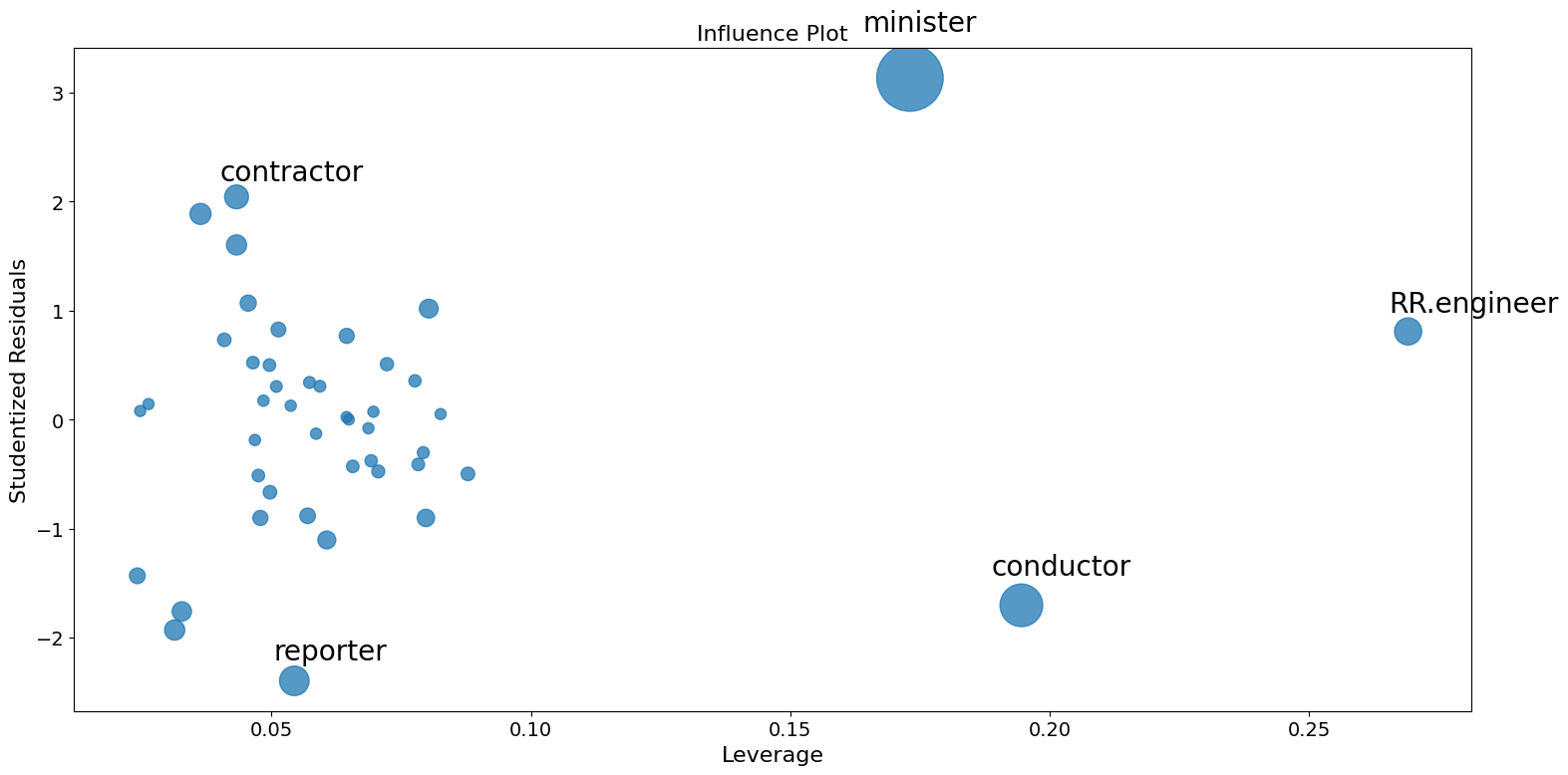
ご覧のとおり、いくつかの懸念すべき観測値があります。contractorとreporterはどちらもレバレッジが低いものの、残差が大きい。RR.engineerは残差が小さく、レバレッジが大きい。Conductorとministerは、レバレッジと残差の両方が大きいため、影響度が大きい。
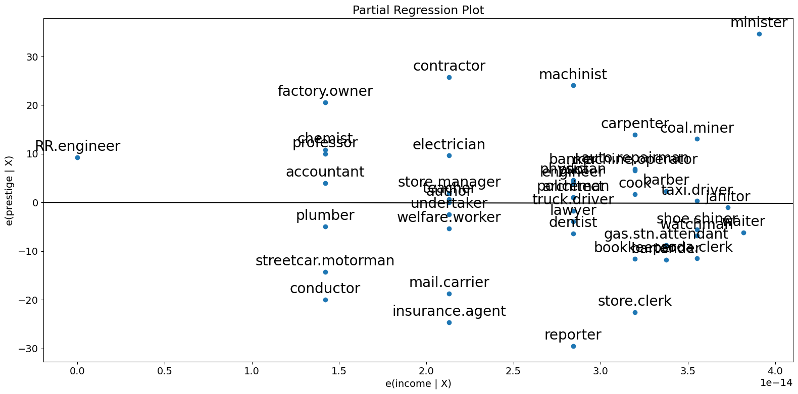
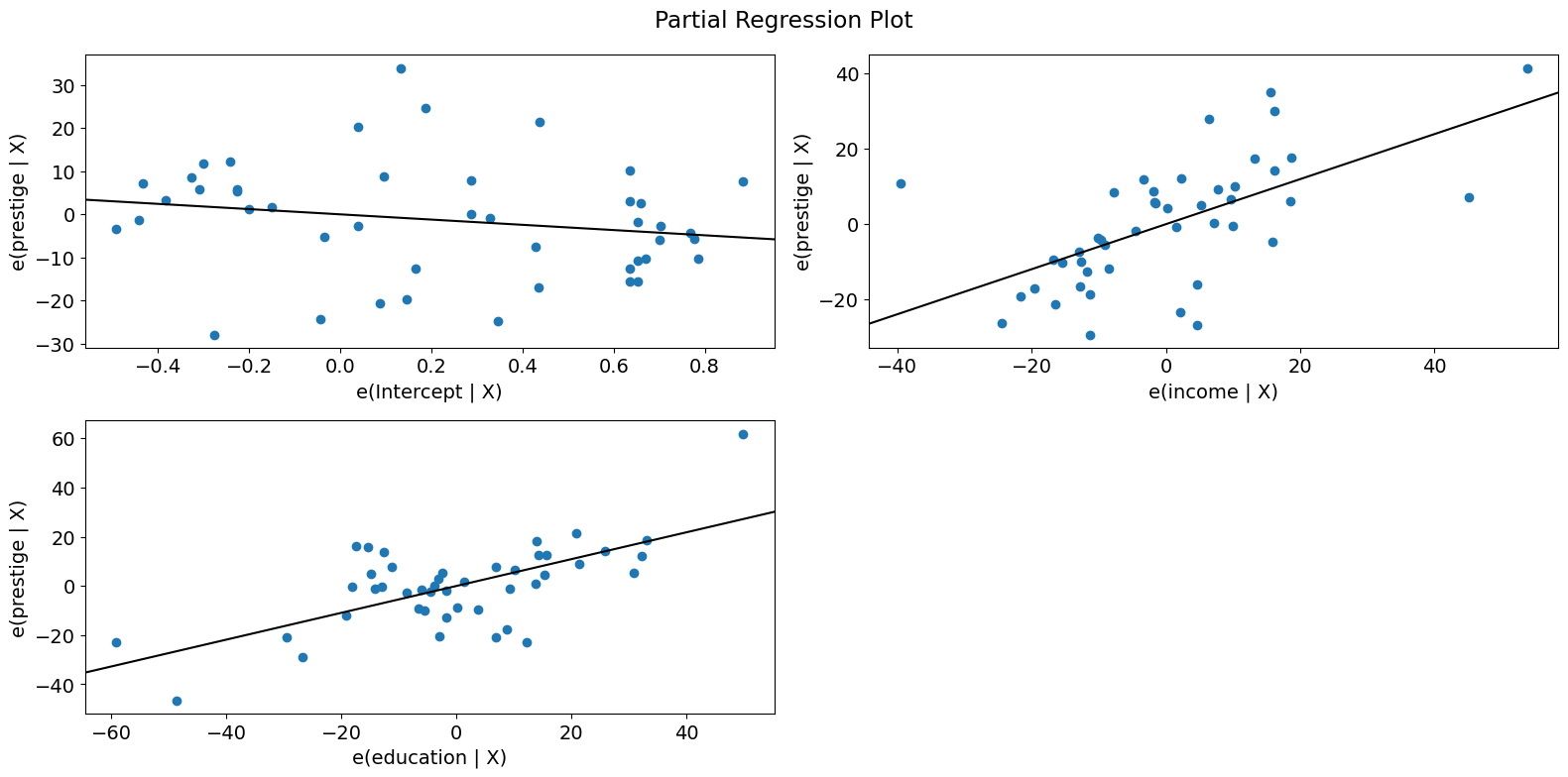
部分回帰プロット (ダンカン)
多変量回帰を行っているため、関係性を識別するために個別の二変量プロットを見るだけでは不十分です。代わりに、他の独立変数に対する条件付きで、従属変数と独立変数の関係を見たいと考えます。これは、部分回帰プロット、別名加変数プロットを使用することで実行できます。
部分回帰プロットでは、応答変数と \(k\) 番目の変数の関係を識別するために、応答変数を \(X_k\) を除く独立変数に対して回帰することにより、残差を計算します。これを \(X_{\sim k}\) で表すことができます。次に、\(X_k\) を \(X_{\sim k}\) に回帰して残差を計算します。部分回帰プロットは、前者の残差と後者の残差のプロットです。
このプロットの注目すべき点は、適合線の傾きが \(\beta_k\) であり、切片がゼロであることです。このプロットの残差は、完全な \(X\) を持つ元のモデルの最小二乗適合の残差と同じです。個々のデータ値が係数の推定に与える影響を容易に識別できます。obs_labelsがTrueの場合、これらの点は観測ラベルで注釈が付けられます。また、等分散性や線形性などの前提条件の違反も確認できます。
[8]:
fig = sm.graphics.plot_partregress(
    "prestige", "income", ["income", "education"], data=prestige
)
fig.tight_layout(pad=1.0)
[9]:
fig = sm.graphics.plot_partregress("prestige", "income", ["education"], data=prestige)
fig.tight_layout(pad=1.0)
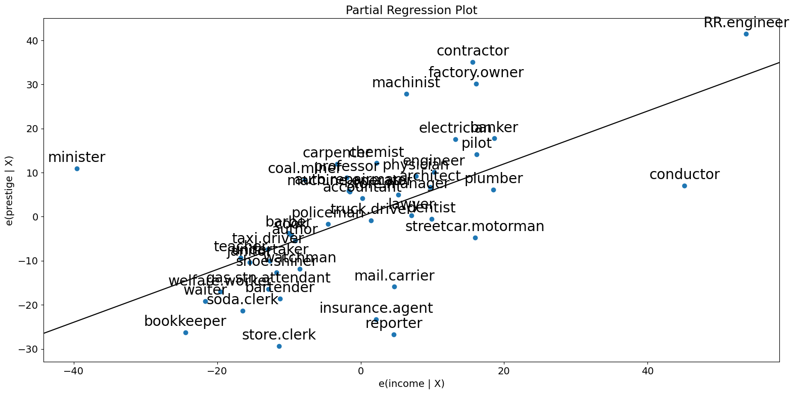
ご覧のとおり、部分回帰プロットは、incomeとprestigeの部分的な関係に対するconductor、minister、およびRR.engineerの影響を確認します。これらのケースは、所得が威信に与える影響を大幅に減少させます。これらのケースを削除すると、これが確認できます。
[10]:
subset = ~prestige.index.isin(["conductor", "RR.engineer", "minister"])
prestige_model2 = ols(
    "prestige ~ income + education", data=prestige, subset=subset
).fit()
print(prestige_model2.summary())
                            OLS Regression Results
==============================================================================
Dep. Variable:               prestige   R-squared:                       0.876
Model:                            OLS   Adj. R-squared:                  0.870
Method:                 Least Squares   F-statistic:                     138.1
Date:                Thu, 03 Oct 2024   Prob (F-statistic):           2.02e-18
Time:                        15:58:28   Log-Likelihood:                -160.59
No. Observations:                  42   AIC:                             327.2
Df Residuals:                      39   BIC:                             332.4
Df Model:                           2
Covariance Type:            nonrobust
==============================================================================
                 coef    std err          t      P>|t|      [0.025      0.975]
------------------------------------------------------------------------------
Intercept     -6.3174      3.680     -1.717      0.094     -13.760       1.125
income         0.9307      0.154      6.053      0.000       0.620       1.242
education      0.2846      0.121      2.345      0.024       0.039       0.530
==============================================================================
Omnibus:                        3.811   Durbin-Watson:                   1.468
Prob(Omnibus):                  0.149   Jarque-Bera (JB):                2.802
Skew:                          -0.614   Prob(JB):                        0.246
Kurtosis:                       3.303   Cond. No.                         158.
==============================================================================

Notes:
[1] Standard Errors assume that the covariance matrix of the errors is correctly specified.
すべての回帰変数をすばやく確認するには、plot_partregress_gridを使用できます。これらのプロットは点にラベルを付けませんが、問題点を特定し、plot_partregressを使用して詳細情報を取得できます。
[11]:
fig = sm.graphics.plot_partregress_grid(prestige_model)
fig.tight_layout(pad=1.0)
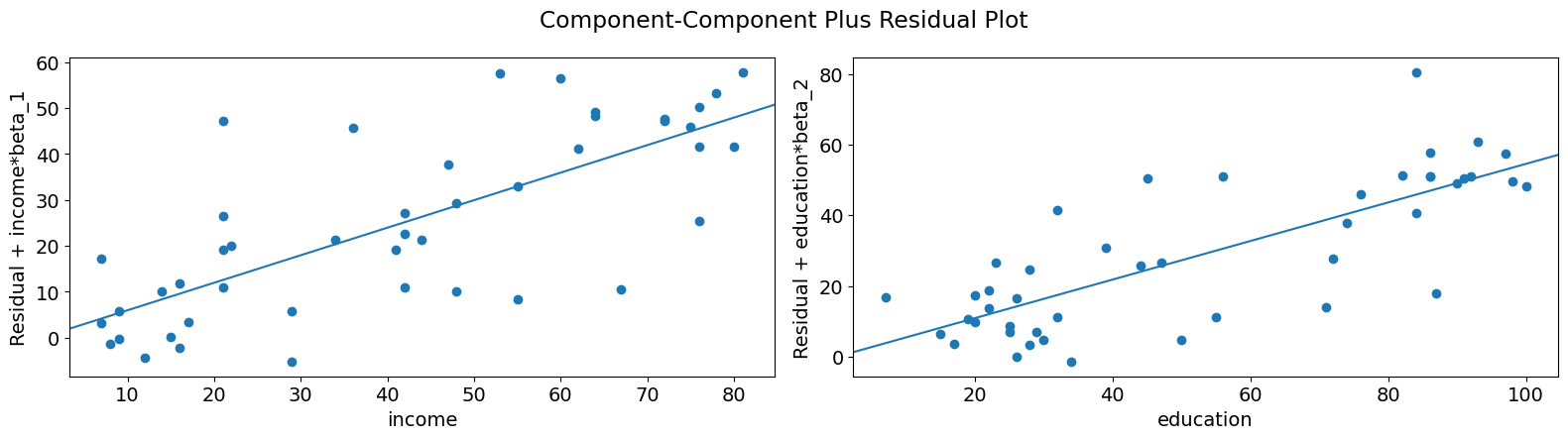
成分-成分プラス残差 (CCPR) プロット
CCPRプロットは、他の独立変数の影響を考慮して、1つの回帰変数が応答変数に与える影響を判断する方法を提供します。部分残差プロットは、\(\text{Residuals} + B_iX_i \text{ }\text{ }\) 対 \(X_i\) として定義されます。成分は、適合線がどこにあるかを示すために、\(B_iX_i\) 対 \(X_i\) を追加します。\(X_i\) が他の独立変数のいずれかと高い相関関係にある場合は注意が必要です。その場合、プロットで明らかになる分散は、真の分散を過小評価することになります。
[12]:
fig = sm.graphics.plot_ccpr(prestige_model, "education")
fig.tight_layout(pad=1.0)
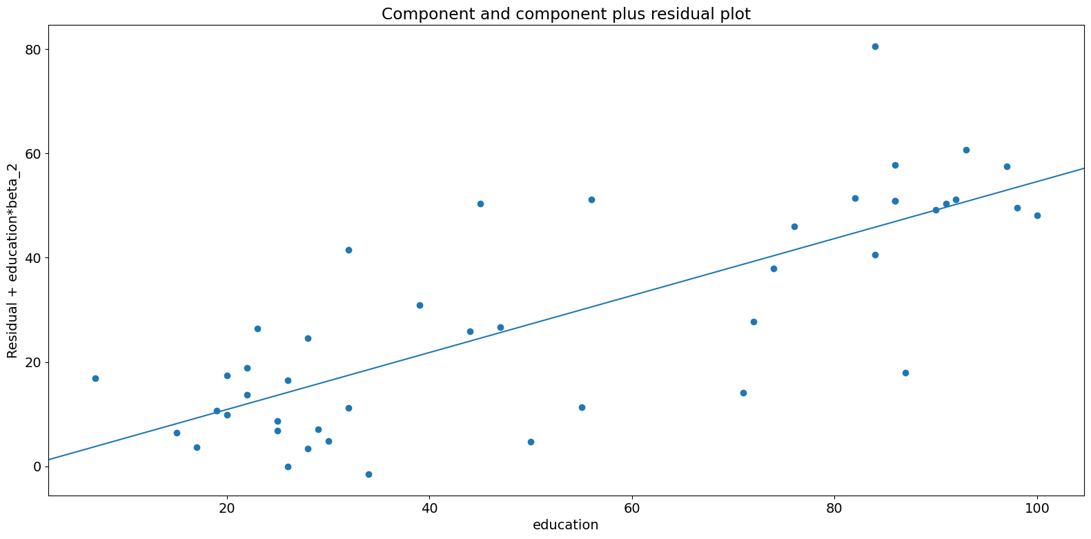
ご覧のとおり、所得を条件とした教育によって説明される威信の変動の関係は線形であるようですが、その関係にかなりの影響を与えているいくつかの観測値があることがわかります。plot_ccpr_gridを使用して、複数の変数をすばやく見ることができます。
[13]:
fig = sm.graphics.plot_ccpr_grid(prestige_model)
fig.tight_layout(pad=1.0)
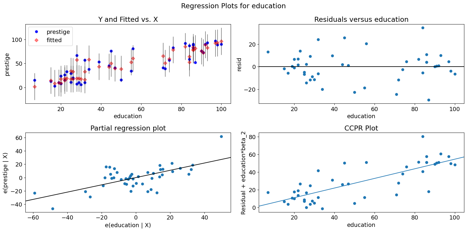
単一変数回帰診断
plot_regress_exog関数は、選択した独立変数に対する従属変数と信頼区間付きの適合値、選択した独立変数に対するモデルの残差、部分回帰プロット、およびCCPRプロットを含む2x2プロットを提供する便利な関数です。この関数は、単一の回帰変数に関してモデリングの前提をすばやく確認するために使用できます。
[14]:
fig = sm.graphics.plot_regress_exog(prestige_model, "education")
fig.tight_layout(pad=1.0)
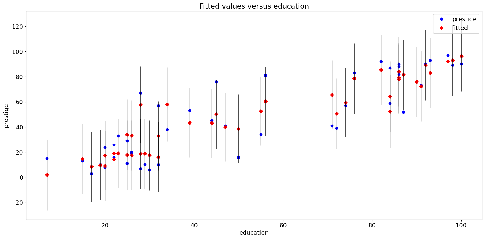
適合プロット
plot_fit関数は、選択した独立変数に対する適合値をプロットします。これには、予測信頼区間が含まれており、必要に応じて真の従属変数をプロットします。
[15]:
fig = sm.graphics.plot_fit(prestige_model, "education")
fig.tight_layout(pad=1.0)
2009年の州別犯罪データセット
http://www.ats.ucla.edu/stat/stata/webbooks/reg/chapter4/statareg_self_assessment_answers4.htm と以下を比較してください。
ただし、ここでのデータは、その例のデータと同じではありません。以下の必要なセルをコメント解除することで、その例を実行できます。
[16]:
# dta = pd.read_csv("http://www.stat.ufl.edu/~aa/social/csv_files/statewide-crime-2.csv")
# dta = dta.set_index("State", inplace=True).dropna()
# dta.rename(columns={"VR" : "crime",
#                    "MR" : "murder",
#                    "M"  : "pctmetro",
#                    "W"  : "pctwhite",
#                    "H"  : "pcths",
#                    "P"  : "poverty",
#                    "S"  : "single"
#                    }, inplace=True)
#
# crime_model = ols("murder ~ pctmetro + poverty + pcths + single", data=dta).fit()
[17]:
dta = sm.datasets.statecrime.load_pandas().data
[18]:
crime_model = ols("murder ~ urban + poverty + hs_grad + single", data=dta).fit()
print(crime_model.summary())
                            OLS Regression Results
==============================================================================
Dep. Variable:                 murder   R-squared:                       0.813
Model:                            OLS   Adj. R-squared:                  0.797
Method:                 Least Squares   F-statistic:                     50.08
Date:                Thu, 03 Oct 2024   Prob (F-statistic):           3.42e-16
Time:                        15:58:34   Log-Likelihood:                -95.050
No. Observations:                  51   AIC:                             200.1
Df Residuals:                      46   BIC:                             209.8
Df Model:                           4
Covariance Type:            nonrobust
==============================================================================
                 coef    std err          t      P>|t|      [0.025      0.975]
------------------------------------------------------------------------------
Intercept    -44.1024     12.086     -3.649      0.001     -68.430     -19.774
urban          0.0109      0.015      0.707      0.483      -0.020       0.042
poverty        0.4121      0.140      2.939      0.005       0.130       0.694
hs_grad        0.3059      0.117      2.611      0.012       0.070       0.542
single         0.6374      0.070      9.065      0.000       0.496       0.779
==============================================================================
Omnibus:                        1.618   Durbin-Watson:                   2.507
Prob(Omnibus):                  0.445   Jarque-Bera (JB):                0.831
Skew:                          -0.220   Prob(JB):                        0.660
Kurtosis:                       3.445   Cond. No.                     5.80e+03
==============================================================================

Notes:
[1] Standard Errors assume that the covariance matrix of the errors is correctly specified.
[2] The condition number is large, 5.8e+03. This might indicate that there are
strong multicollinearity or other numerical problems.
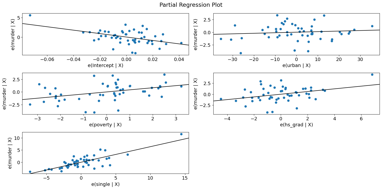
部分回帰プロット (犯罪データ)
[19]:
fig = sm.graphics.plot_partregress_grid(crime_model)
fig.tight_layout(pad=1.0)
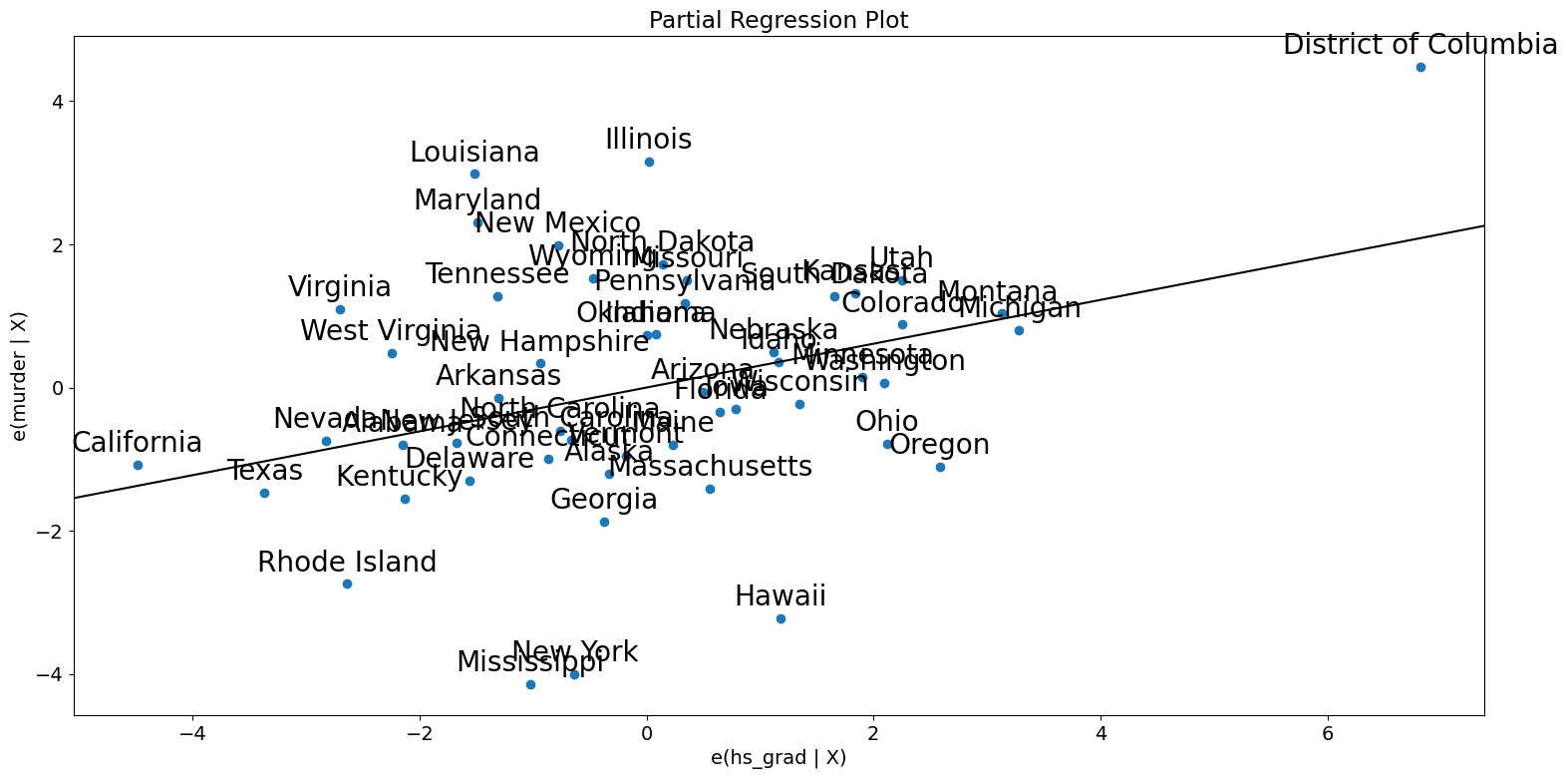
[20]:
fig = sm.graphics.plot_partregress(
    "murder", "hs_grad", ["urban", "poverty", "single"], data=dta
)
fig.tight_layout(pad=1.0)
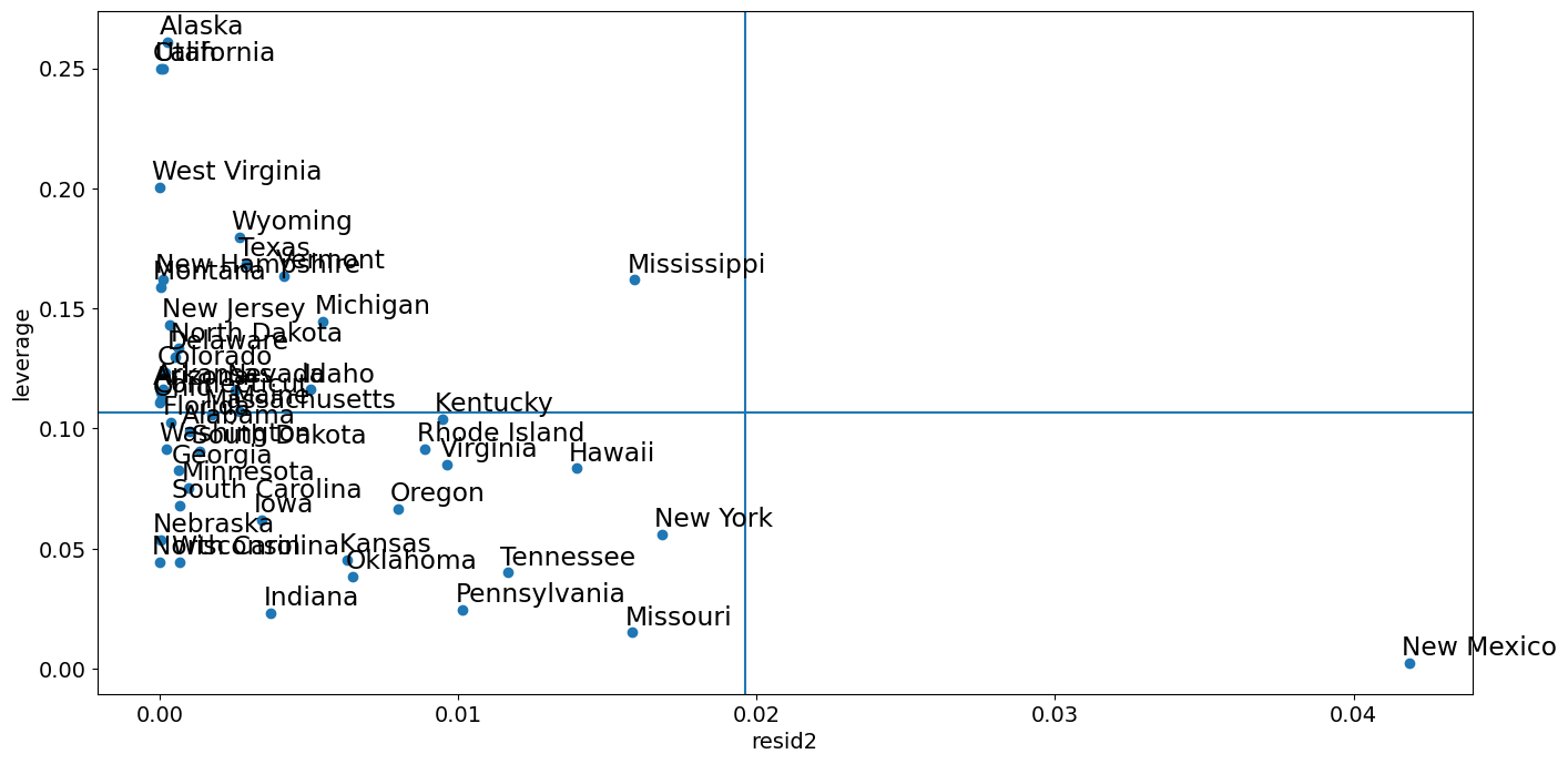
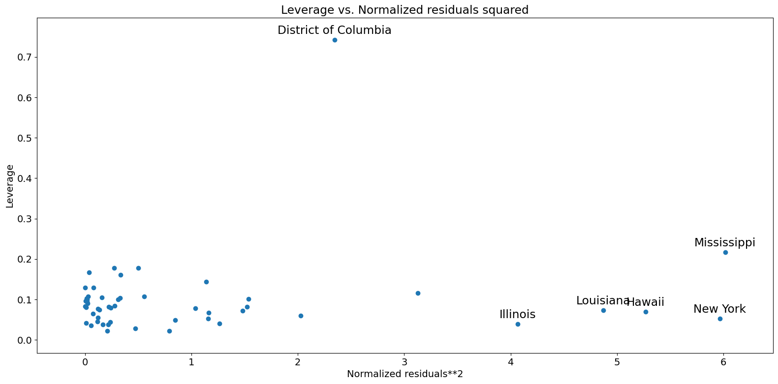
レバレッジ-残差二乗プロット
influence_plotと密接に関連しているのが、レバレッジ-残差二乗プロットです。
[21]:
fig = sm.graphics.plot_leverage_resid2(crime_model)
fig.tight_layout(pad=1.0)
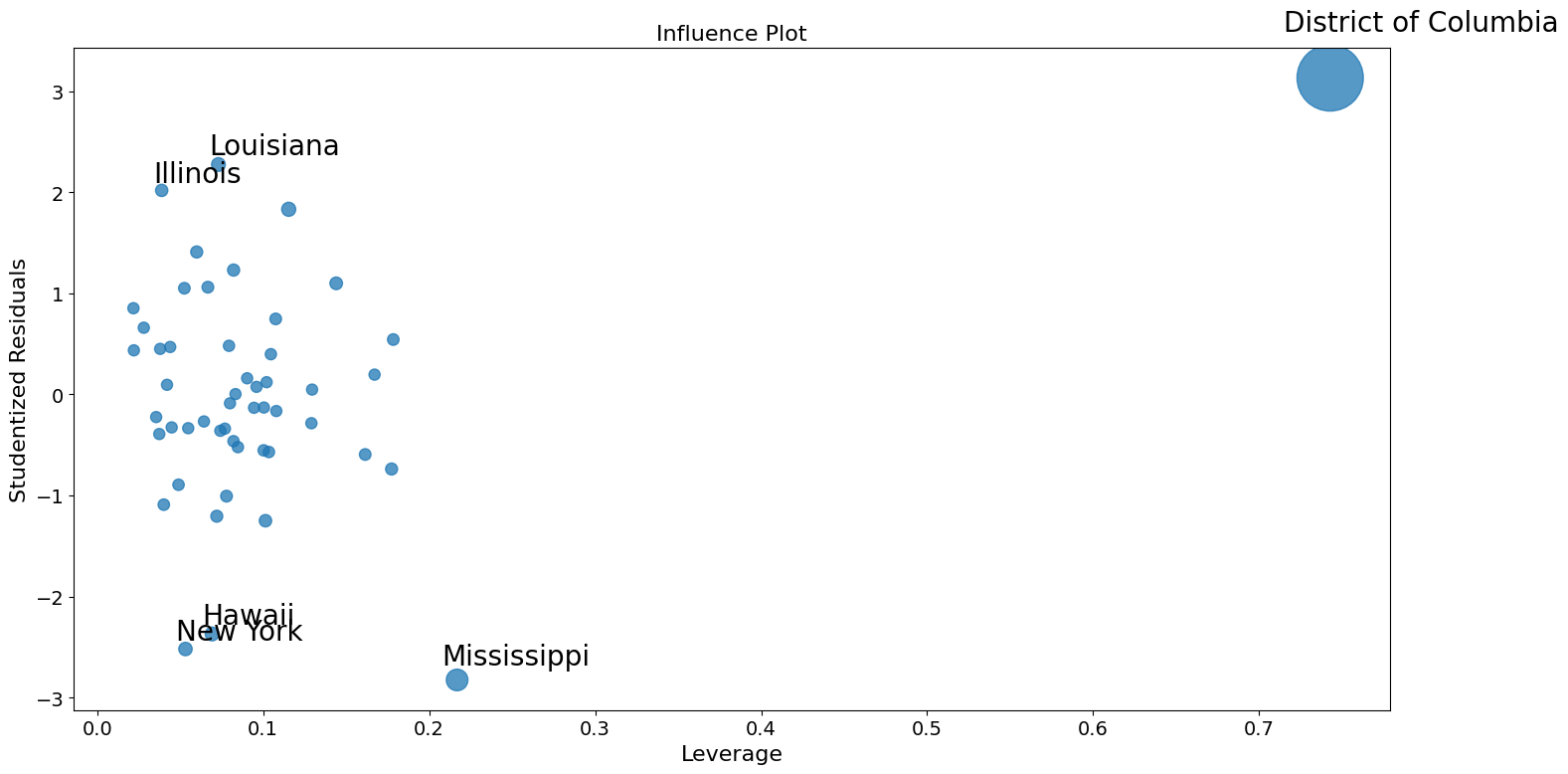
影響度プロット
[22]:
fig = sm.graphics.influence_plot(crime_model)
fig.tight_layout(pad=1.0)
外れ値を修正するためのロバスト回帰の使用
ここでStataの結果を再現する際の問題の一部は、M推定量がレバレッジポイントに対してロバストではないことです。MM推定量はこの例でより効果的であるはずです。
[23]:
from statsmodels.formula.api import rlm
[24]:
rob_crime_model = rlm(
    "murder ~ urban + poverty + hs_grad + single",
    data=dta,
    M=sm.robust.norms.TukeyBiweight(3),
).fit(conv="weights")
print(rob_crime_model.summary())
                    Robust linear Model Regression Results
==============================================================================
Dep. Variable:                 murder   No. Observations:                   51
Model:                            RLM   Df Residuals:                       46
Method:                          IRLS   Df Model:                            4
Norm:                   TukeyBiweight
Scale Est.:                       mad
Cov Type:                          H1
Date:                Thu, 03 Oct 2024
Time:                        15:58:38
No. Iterations:                    50
==============================================================================
                 coef    std err          z      P>|z|      [0.025      0.975]
------------------------------------------------------------------------------
Intercept     -4.2986      9.494     -0.453      0.651     -22.907      14.310
urban          0.0029      0.012      0.241      0.809      -0.021       0.027
poverty        0.2753      0.110      2.499      0.012       0.059       0.491
hs_grad       -0.0302      0.092     -0.328      0.743      -0.211       0.150
single         0.2902      0.055      5.253      0.000       0.182       0.398
==============================================================================

If the model instance has been used for another fit with different fit parameters, then the fit options might not be the correct ones anymore .
[25]:
# rob_crime_model = rlm("murder ~ pctmetro + poverty + pcths + single", data=dta, M=sm.robust.norms.TukeyBiweight()).fit(conv="weights")
# print(rob_crime_model.summary())
RLMの一部としてまだ影響診断方法は存在しませんが、それらを再現できます。(これは、issue #888 のステータスに依存します。)
[26]:
weights = rob_crime_model.weights
idx = weights > 0
X = rob_crime_model.model.exog[idx.values]
ww = weights[idx] / weights[idx].mean()
hat_matrix_diag = ww * (X * np.linalg.pinv(X).T).sum(1)
resid = rob_crime_model.resid
resid2 = resid ** 2
resid2 /= resid2.sum()
nobs = int(idx.sum())
hm = hat_matrix_diag.mean()
rm = resid2.mean()
[27]:
from statsmodels.graphics import utils

fig, ax = plt.subplots(figsize=(16, 8))
ax.plot(resid2[idx], hat_matrix_diag, "o")
ax = utils.annotate_axes(
    range(nobs),
    labels=rob_crime_model.model.data.row_labels[idx],
    points=lzip(resid2[idx], hat_matrix_diag),
    offset_points=[(-5, 5)] * nobs,
    size="large",
    ax=ax,
)
ax.set_xlabel("resid2")
ax.set_ylabel("leverage")
ylim = ax.get_ylim()
ax.vlines(rm, *ylim)
xlim = ax.get_xlim()
ax.hlines(hm, *xlim)
ax.margins(0, 0)