シータモデル
Assimakopoulos & Nikolopoulos (2000) のシータモデルは、2本のθ線をフィッティングし、単純指数平滑化を用いて線を予測し、2本の線の予測を組み合わせて最終的な予測を生成する、単純な予測手法です。このモデルは段階的に実装されます。
季節性の検定
季節性が検出された場合、季節調整を行う
データにSESモデルをフィッティングすることでαを推定し、OLSを用いてb₀を推定する。
時系列を予測する
データが季節調整された場合は、再季節調整を行う。
季節性の検定では、季節ラグmにおけるACFを調べます。このラグがゼロと有意に異なる場合、データはstatsmodels.tsa.seasonal_decomposeを用いて季節調整されます。乗法モデル(デフォルト)または加法モデルを使用できます。
このモデルのパラメータはb₀とαであり、b₀はOLS回帰
から推定され、αは
におけるSES平滑化パラメータです。予測値は
となります。最終的に、θはトレンドがどれだけ減衰するかを決定する役割しか果たしません。θが非常に大きい場合、このモデルの予測はドリフトのある積分移動平均
からの予測と同じになります。最後に、必要に応じて予測値を再季節調整します。
このモジュールは以下に基づいています。
Assimakopoulos, V., & Nikolopoulos, K. (2000). The theta model: a decomposition approach to forecasting. International journal of forecasting, 16(4), 521-530.
Hyndman, R. J., & Billah, B. (2003). Unmasking the Theta method. International Journal of Forecasting, 19(2), 287-290.
Fioruci, J. A., Pellegrini, T. R., Louzada, F., & Petropoulos, F. (2015). The optimized theta method. arXiv preprint arXiv:1503.03529.
インポート
標準的なインポートセットと、デフォルトのmatplotlibスタイルの微調整から始めます。
[1]:
import matplotlib.pyplot as plt
import numpy as np
import pandas as pd
import pandas_datareader as pdr
import seaborn as sns

plt.rc("figure", figsize=(16, 8))
plt.rc("font", size=15)
plt.rc("lines", linewidth=3)
sns.set_style("darkgrid")
データの読み込み
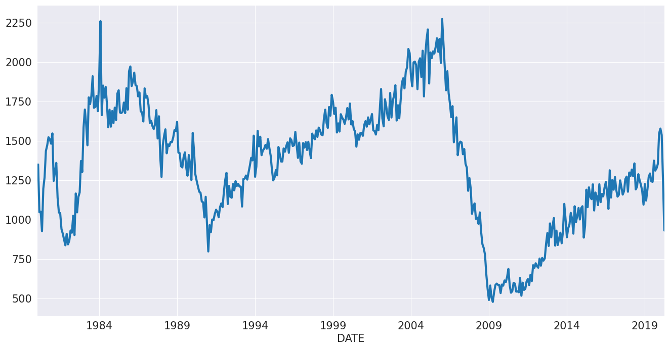
最初に、米国データを使用して住宅着工件数を見てみましょう。この時系列は明らかに季節性がありますが、同じ期間中に明確なトレンドはありません。
[2]:
reader = pdr.fred.FredReader(["HOUST"], start="1980-01-01", end="2020-04-01")
data = reader.read()
housing = data.HOUST
housing.index.freq = housing.index.inferred_freq
ax = housing.plot()
オプションなしでモデルを指定し、フィッティングします。サマリーは、データが乗法モデルを使用して季節調整されたことを示しています。ドリフトは控えめで負であり、平滑化パラメータは非常に低くなっています。
[3]:
from statsmodels.tsa.forecasting.theta import ThetaModel

tm = ThetaModel(housing)
res = tm.fit()
print(res.summary())
                              ThetaModel Results
==============================================================================
Dep. Variable:                  HOUST   No. Observations:                  484
Method:                       OLS/SES   Deseasonalized:                   True
Date:                Thu, 03 Oct 2024   Deseas. Method:         Multiplicative
Time:                        15:46:28   Period:                             12
Sample:                    01-01-1980
                         - 04-01-2020
   Parameter Estimates
=========================
           Parameters
-------------------------
b0    -0.9194460961668147
alpha   0.616996789006705
-------------------------
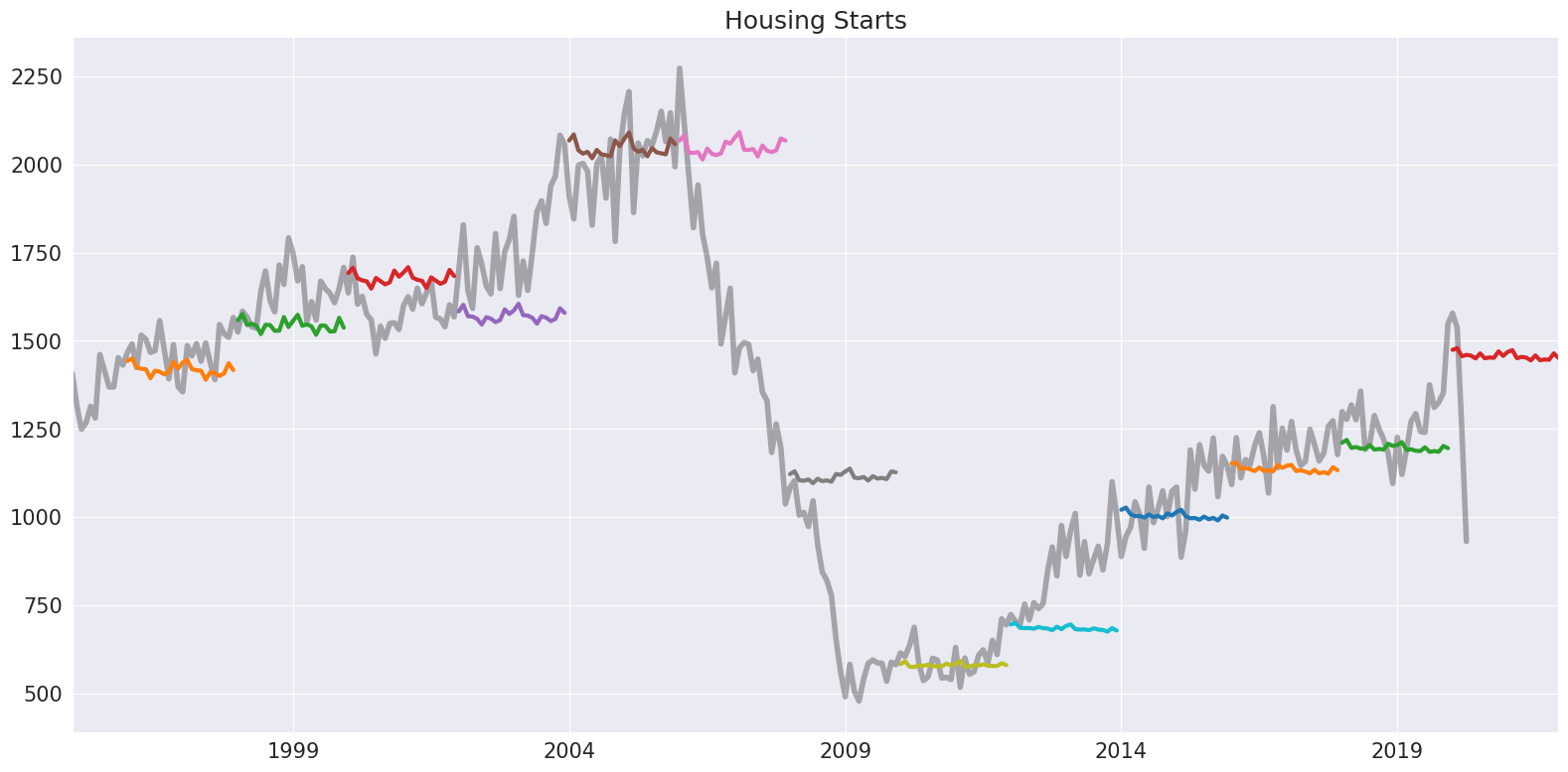
このモデルは、何よりもまず予測手法です。予測は、フィッティングされたモデルからforecastメソッドを使用して生成されます。以下では、2年先を2年ごとに予測することによって、ハリネズミプロットを作成します。
**注記**: デフォルトのθは2です。
[4]:
forecasts = {"housing": housing}
for year in range(1995, 2020, 2):
    sub = housing[: str(year)]
    res = ThetaModel(sub).fit()
    fcast = res.forecast(24)
    forecasts[str(year)] = fcast
forecasts = pd.DataFrame(forecasts)
ax = forecasts["1995":].plot(legend=False)
children = ax.get_children()
children[0].set_linewidth(4)
children[0].set_alpha(0.3)
children[0].set_color("#000000")
ax.set_title("Housing Starts")
plt.tight_layout(pad=1.0)
代わりに、データの対数をとってフィッティングすることもできます。ここでは、必要に応じて、季節調整に加法モデルを使用することを強制する方が理にかなっています。また、MLEを使用してモデルパラメータをフィッティングします。この方法は、IMA
をフィッティングします。ここで、\(\hat{\alpha}\) = \(\min(\hat{\gamma}+1, 0.9998)\)であり、statsmodels.tsa.SARIMAXを使用します。パラメータは似ていますが、ドリフトはゼロに近くなっています。
[5]:
tm = ThetaModel(np.log(housing), method="additive")
res = tm.fit(use_mle=True)
print(res.summary())
                              ThetaModel Results
==============================================================================
Dep. Variable:                  HOUST   No. Observations:                  484
Method:                           MLE   Deseasonalized:                   True
Date:                Thu, 03 Oct 2024   Deseas. Method:               Additive
Time:                        15:46:30   Period:                             12
Sample:                    01-01-1980
                         - 04-01-2020
     Parameter Estimates
=============================
             Parameters
-----------------------------
b0    -0.00044644118691643226
alpha       0.670610385005854
-----------------------------
予測は、予測トレンドコンポーネント
SESからの予測(予測期間とは変化しない)、および季節性にのみ依存します。これら3つのコンポーネントは、forecast_componentsを使用して利用できます。これにより、上記の重み式を使用して、複数のθの選択を使用して予測を作成できます。
[6]:
res.forecast_components(12)
[6]:
| トレンド | SES | 季節性 | |
|---|---|---|---|
| 2020-05-01 | -0.000666 | 6.95726 | -0.001252 |
| 2020-06-01 | -0.001112 | 6.95726 | -0.006891 |
| 2020-07-01 | -0.001559 | 6.95726 | 0.002992 |
| 2020-08-01 | -0.002005 | 6.95726 | -0.003817 |
| 2020-09-01 | -0.002451 | 6.95726 | -0.003902 |
| 2020-10-01 | -0.002898 | 6.95726 | -0.003981 |
| 2020-11-01 | -0.003344 | 6.95726 | 0.008536 |
| 2020-12-01 | -0.003791 | 6.95726 | -0.000714 |
| 2021-01-01 | -0.004237 | 6.95726 | 0.005239 |
| 2021-02-01 | -0.004684 | 6.95726 | 0.009943 |
| 2021-03-01 | -0.005130 | 6.95726 | -0.004535 |
| 2021-04-01 | -0.005577 | 6.95726 | -0.001619 |
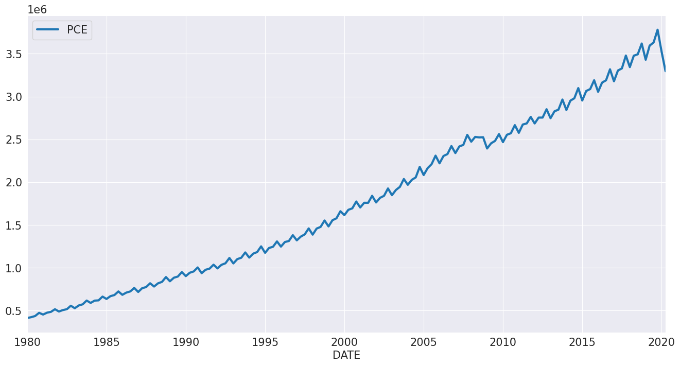
個人消費支出
次に、個人消費支出を見てみましょう。この時系列には、明確な季節成分とドリフトがあります。
[7]:
reader = pdr.fred.FredReader(["NA000349Q"], start="1980-01-01", end="2020-04-01")
pce = reader.read()
pce.columns = ["PCE"]
pce.index.freq = "QS-OCT"
_ = pce.plot()
この時系列は常に正なので、lnをモデル化します。
[8]:
mod = ThetaModel(np.log(pce))
res = mod.fit()
print(res.summary())
                              ThetaModel Results
==============================================================================
Dep. Variable:                    PCE   No. Observations:                  162
Method:                       OLS/SES   Deseasonalized:                   True
Date:                Thu, 03 Oct 2024   Deseas. Method:         Multiplicative
Time:                        15:46:32   Period:                              4
Sample:                    01-01-1980
                         - 04-01-2020
   Parameter Estimates
==========================
           Parameters
--------------------------
b0    0.013035370221488518
alpha   0.9998851279204637
--------------------------
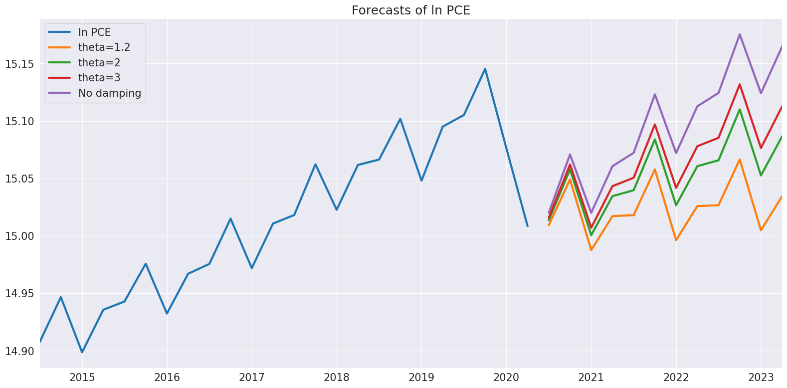
次に、θが変化する際の予測の差を調べます。θが1に近い場合、ドリフトはほとんど存在しません。θが増加するにつれて、ドリフトはより顕著になります。
[9]:
forecasts = pd.DataFrame(
    {
        "ln PCE": np.log(pce.PCE),
        "theta=1.2": res.forecast(12, theta=1.2),
        "theta=2": res.forecast(12),
        "theta=3": res.forecast(12, theta=3),
        "No damping": res.forecast(12, theta=np.inf),
    }
)
_ = forecasts.tail(36).plot()
plt.title("Forecasts of ln PCE")
plt.tight_layout(pad=1.0)
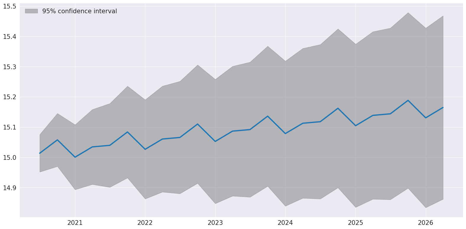
最後に、plot_predictを使用して、予測と予測区間を視覚化できます。予測区間は、IMAが真であると仮定して構築されます。
[10]:
ax = res.plot_predict(24, theta=2)
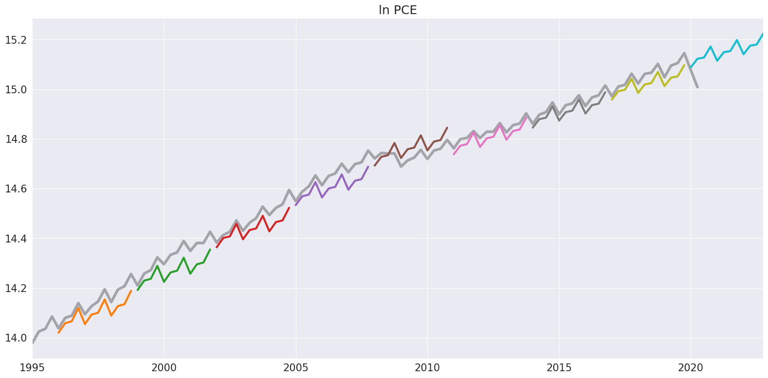
2年間の非重複サンプルを使用してハリネズミプロットを作成することで結論付けます。
[11]:
ln_pce = np.log(pce.PCE)
forecasts = {"ln PCE": ln_pce}
for year in range(1995, 2020, 3):
    sub = ln_pce[: str(year)]
    res = ThetaModel(sub).fit()
    fcast = res.forecast(12)
    forecasts[str(year)] = fcast
forecasts = pd.DataFrame(forecasts)
ax = forecasts["1995":].plot(legend=False)
children = ax.get_children()
children[0].set_linewidth(4)
children[0].set_alpha(0.3)
children[0].set_color("#000000")
ax.set_title("ln PCE")
plt.tight_layout(pad=1.0)