最小二乗法
[1]:
%matplotlib inline
[2]:
import matplotlib.pyplot as plt
import numpy as np
import pandas as pd
import statsmodels.api as sm

np.random.seed(9876789)
OLS推定
人工データ
[3]:
nsample = 100
x = np.linspace(0, 10, 100)
X = np.column_stack((x, x ** 2))
beta = np.array([1, 0.1, 10])
e = np.random.normal(size=nsample)
モデルには切片が必要なので、1の列を追加します。
[4]:
X = sm.add_constant(X)
y = np.dot(X, beta) + e
適合とサマリー
[5]:
model = sm.OLS(y, X)
results = model.fit()
print(results.summary())
                            OLS Regression Results
==============================================================================
Dep. Variable:                      y   R-squared:                       1.000
Model:                            OLS   Adj. R-squared:                  1.000
Method:                 Least Squares   F-statistic:                 4.020e+06
Date:                Thu, 03 Oct 2024   Prob (F-statistic):          2.83e-239
Time:                        15:44:50   Log-Likelihood:                -146.51
No. Observations:                 100   AIC:                             299.0
Df Residuals:                      97   BIC:                             306.8
Df Model:                           2
Covariance Type:            nonrobust
==============================================================================
                 coef    std err          t      P>|t|      [0.025      0.975]
------------------------------------------------------------------------------
const          1.3423      0.313      4.292      0.000       0.722       1.963
x1            -0.0402      0.145     -0.278      0.781      -0.327       0.247
x2            10.0103      0.014    715.745      0.000       9.982      10.038
==============================================================================
Omnibus:                        2.042   Durbin-Watson:                   2.274
Prob(Omnibus):                  0.360   Jarque-Bera (JB):                1.875
Skew:                           0.234   Prob(JB):                        0.392
Kurtosis:                       2.519   Cond. No.                         144.
==============================================================================

Notes:
[1] Standard Errors assume that the covariance matrix of the errors is correctly specified.
関心のある量は、適合済みモデルから直接抽出できます。dir(results)と入力すると、完全なリストが表示されます。いくつかの例を以下に示します。
[6]:
print("Parameters: ", results.params)
print("R2: ", results.rsquared)
Parameters:  [ 1.34233516 -0.04024948 10.01025357]
R2:  0.9999879365025871
OLS非線形曲線だがパラメータに関して線形
xとyの間に非線形関係を持つ人工データをシミュレートします。
[7]:
nsample = 50
sig = 0.5
x = np.linspace(0, 20, nsample)
X = np.column_stack((x, np.sin(x), (x - 5) ** 2, np.ones(nsample)))
beta = [0.5, 0.5, -0.02, 5.0]

y_true = np.dot(X, beta)
y = y_true + sig * np.random.normal(size=nsample)
適合とサマリー
[8]:
res = sm.OLS(y, X).fit()
print(res.summary())
                            OLS Regression Results
==============================================================================
Dep. Variable:                      y   R-squared:                       0.933
Model:                            OLS   Adj. R-squared:                  0.928
Method:                 Least Squares   F-statistic:                     211.8
Date:                Thu, 03 Oct 2024   Prob (F-statistic):           6.30e-27
Time:                        15:44:50   Log-Likelihood:                -34.438
No. Observations:                  50   AIC:                             76.88
Df Residuals:                      46   BIC:                             84.52
Df Model:                           3
Covariance Type:            nonrobust
==============================================================================
                 coef    std err          t      P>|t|      [0.025      0.975]
------------------------------------------------------------------------------
x1             0.4687      0.026     17.751      0.000       0.416       0.522
x2             0.4836      0.104      4.659      0.000       0.275       0.693
x3            -0.0174      0.002     -7.507      0.000      -0.022      -0.013
const          5.2058      0.171     30.405      0.000       4.861       5.550
==============================================================================
Omnibus:                        0.655   Durbin-Watson:                   2.896
Prob(Omnibus):                  0.721   Jarque-Bera (JB):                0.360
Skew:                           0.207   Prob(JB):                        0.835
Kurtosis:                       3.026   Cond. No.                         221.
==============================================================================

Notes:
[1] Standard Errors assume that the covariance matrix of the errors is correctly specified.
関心のある他の量を抽出します。
[9]:
print("Parameters: ", res.params)
print("Standard errors: ", res.bse)
print("Predicted values: ", res.predict())
Parameters:  [ 0.46872448  0.48360119 -0.01740479  5.20584496]
Standard errors:  [0.02640602 0.10380518 0.00231847 0.17121765]
Predicted values:  [ 4.77072516  5.22213464  5.63620761  5.98658823  6.25643234  6.44117491
  6.54928009  6.60085051  6.62432454  6.6518039   6.71377946  6.83412169
  7.02615877  7.29048685  7.61487206  7.97626054  8.34456611  8.68761335
  8.97642389  9.18997755  9.31866582  9.36587056  9.34740836  9.28893189
  9.22171529  9.17751587  9.1833565   9.25708583  9.40444579  9.61812821
  9.87897556 10.15912843 10.42660281 10.65054491 10.8063004  10.87946503
 10.86825119 10.78378163 10.64826203 10.49133265 10.34519853 10.23933827
 10.19566084 10.22490593 10.32487947 10.48081414 10.66779556 10.85485568
 11.01006072 11.10575781]
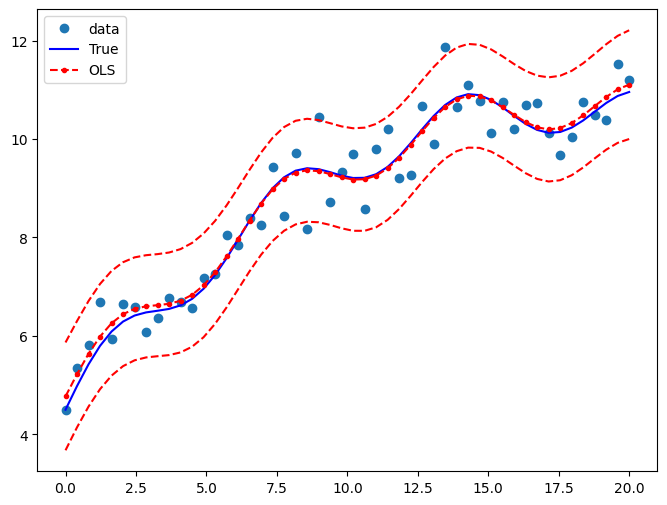
真の関係とOLS予測を比較するためのプロットを描画します。予測値の信頼区間は、wls_prediction_stdコマンドを使用して構築されます。
[10]:
pred_ols = res.get_prediction()
iv_l = pred_ols.summary_frame()["obs_ci_lower"]
iv_u = pred_ols.summary_frame()["obs_ci_upper"]

fig, ax = plt.subplots(figsize=(8, 6))

ax.plot(x, y, "o", label="data")
ax.plot(x, y_true, "b-", label="True")
ax.plot(x, res.fittedvalues, "r--.", label="OLS")
ax.plot(x, iv_u, "r--")
ax.plot(x, iv_l, "r--")
ax.legend(loc="best")
[10]:
<matplotlib.legend.Legend at 0x7fe3f3907c70>
ダミー変数を使用したOLS
人工データを作成します。ダミー変数を使用してモデル化される3つのグループがあります。グループ0は省略/基準カテゴリです。
[11]:
nsample = 50
groups = np.zeros(nsample, int)
groups[20:40] = 1
groups[40:] = 2
# dummy = (groups[:,None] == np.unique(groups)).astype(float)

dummy = pd.get_dummies(groups).values
x = np.linspace(0, 20, nsample)
# drop reference category
X = np.column_stack((x, dummy[:, 1:]))
X = sm.add_constant(X, prepend=False)

beta = [1.0, 3, -3, 10]
y_true = np.dot(X, beta)
e = np.random.normal(size=nsample)
y = y_true + e
データを確認します。
[12]:
print(X[:5, :])
print(y[:5])
print(groups)
print(dummy[:5, :])
[[0.         0.         0.         1.        ]
 [0.40816327 0.         0.         1.        ]
 [0.81632653 0.         0.         1.        ]
 [1.2244898  0.         0.         1.        ]
 [1.63265306 0.         0.         1.        ]]
[ 9.28223335 10.50481865 11.84389206 10.38508408 12.37941998]
[0 0 0 0 0 0 0 0 0 0 0 0 0 0 0 0 0 0 0 0 1 1 1 1 1 1 1 1 1 1 1 1 1 1 1 1 1
 1 1 1 2 2 2 2 2 2 2 2 2 2]
[[ True False False]
 [ True False False]
 [ True False False]
 [ True False False]
 [ True False False]]
適合とサマリー
[13]:
res2 = sm.OLS(y, X).fit()
print(res2.summary())
                            OLS Regression Results
==============================================================================
Dep. Variable:                      y   R-squared:                       0.978
Model:                            OLS   Adj. R-squared:                  0.976
Method:                 Least Squares   F-statistic:                     671.7
Date:                Thu, 03 Oct 2024   Prob (F-statistic):           5.69e-38
Time:                        15:44:51   Log-Likelihood:                -64.643
No. Observations:                  50   AIC:                             137.3
Df Residuals:                      46   BIC:                             144.9
Df Model:                           3
Covariance Type:            nonrobust
==============================================================================
                 coef    std err          t      P>|t|      [0.025      0.975]
------------------------------------------------------------------------------
x1             0.9999      0.060     16.689      0.000       0.879       1.121
x2             2.8909      0.569      5.081      0.000       1.746       4.036
x3            -3.2232      0.927     -3.477      0.001      -5.089      -1.357
const         10.1031      0.310     32.573      0.000       9.479      10.727
==============================================================================
Omnibus:                        2.831   Durbin-Watson:                   1.998
Prob(Omnibus):                  0.243   Jarque-Bera (JB):                1.927
Skew:                          -0.279   Prob(JB):                        0.382
Kurtosis:                       2.217   Cond. No.                         96.3
==============================================================================

Notes:
[1] Standard Errors assume that the covariance matrix of the errors is correctly specified.
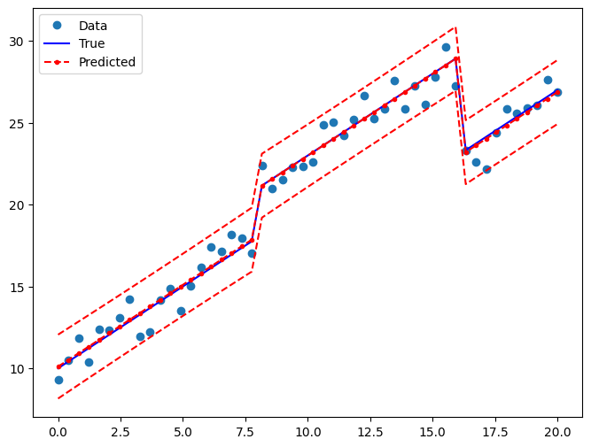
真の関係とOLS予測を比較するためのプロットを描画します。
[14]:
pred_ols2 = res2.get_prediction()
iv_l = pred_ols2.summary_frame()["obs_ci_lower"]
iv_u = pred_ols2.summary_frame()["obs_ci_upper"]

fig, ax = plt.subplots(figsize=(8, 6))

ax.plot(x, y, "o", label="Data")
ax.plot(x, y_true, "b-", label="True")
ax.plot(x, res2.fittedvalues, "r--.", label="Predicted")
ax.plot(x, iv_u, "r--")
ax.plot(x, iv_l, "r--")
legend = ax.legend(loc="best")
同時仮説検定
F検定
ダミー変数の両方の係数がゼロに等しいという仮説、つまり\(R \times \beta = 0\)を検定したいと考えています。F検定により、3つのグループで定数が同一であるという帰無仮説を強く棄却します。
[15]:
R = [[0, 1, 0, 0], [0, 0, 1, 0]]
print(np.array(R))
print(res2.f_test(R))
[[0 1 0 0]
 [0 0 1 0]]
<F test: F=145.49268198027963, p=1.2834419617282974e-20, df_denom=46, df_num=2>
数式のような構文を使用して仮説を検定することもできます。
[16]:
print(res2.f_test("x2 = x3 = 0"))
<F test: F=145.49268198027949, p=1.2834419617283214e-20, df_denom=46, df_num=2>
小グループ効果
より小さなグループ効果を持つ人工データを作成した場合、T検定では帰無仮説を棄却できなくなります。
[17]:
beta = [1.0, 0.3, -0.0, 10]
y_true = np.dot(X, beta)
y = y_true + np.random.normal(size=nsample)

res3 = sm.OLS(y, X).fit()
[18]:
print(res3.f_test(R))
<F test: F=1.224911192540883, p=0.30318644106312964, df_denom=46, df_num=2>
[19]:
print(res3.f_test("x2 = x3 = 0"))
<F test: F=1.2249111925408838, p=0.30318644106312964, df_denom=46, df_num=2>
多重共線性
Longleyデータセットは、多重共線性が高いことでよく知られています。つまり、外生予測変数が高度に相関しています。これは、モデルの仕様をわずかに変更すると係数推定の安定性に影響を与える可能性があるため、問題となります。
[20]:
from statsmodels.datasets.longley import load_pandas

y = load_pandas().endog
X = load_pandas().exog
X = sm.add_constant(X)
適合とサマリー
[21]:
ols_model = sm.OLS(y, X)
ols_results = ols_model.fit()
print(ols_results.summary())
                            OLS Regression Results
==============================================================================
Dep. Variable:                 TOTEMP   R-squared:                       0.995
Model:                            OLS   Adj. R-squared:                  0.992
Method:                 Least Squares   F-statistic:                     330.3
Date:                Thu, 03 Oct 2024   Prob (F-statistic):           4.98e-10
Time:                        15:44:51   Log-Likelihood:                -109.62
No. Observations:                  16   AIC:                             233.2
Df Residuals:                       9   BIC:                             238.6
Df Model:                           6
Covariance Type:            nonrobust
==============================================================================
                 coef    std err          t      P>|t|      [0.025      0.975]
------------------------------------------------------------------------------
const      -3.482e+06    8.9e+05     -3.911      0.004    -5.5e+06   -1.47e+06
GNPDEFL       15.0619     84.915      0.177      0.863    -177.029     207.153
GNP           -0.0358      0.033     -1.070      0.313      -0.112       0.040
UNEMP         -2.0202      0.488     -4.136      0.003      -3.125      -0.915
ARMED         -1.0332      0.214     -4.822      0.001      -1.518      -0.549
POP           -0.0511      0.226     -0.226      0.826      -0.563       0.460
YEAR        1829.1515    455.478      4.016      0.003     798.788    2859.515
==============================================================================
Omnibus:                        0.749   Durbin-Watson:                   2.559
Prob(Omnibus):                  0.688   Jarque-Bera (JB):                0.684
Skew:                           0.420   Prob(JB):                        0.710
Kurtosis:                       2.434   Cond. No.                     4.86e+09
==============================================================================

Notes:
[1] Standard Errors assume that the covariance matrix of the errors is correctly specified.
[2] The condition number is large, 4.86e+09. This might indicate that there are
strong multicollinearity or other numerical problems.
/opt/hostedtoolcache/Python/3.10.15/x64/lib/python3.10/site-packages/scipy/stats/_axis_nan_policy.py:418: UserWarning: `kurtosistest` p-value may be inaccurate with fewer than 20 observations; only n=16 observations were given.
  return hypotest_fun_in(*args, **kwds)
条件数
多重共線性を評価する1つの方法は、条件数を計算することです。20を超える値は懸念事項です(Greene 4.9を参照)。最初のステップは、単位長を持つように独立変数を正規化することです。
[22]:
norm_x = X.values
for i, name in enumerate(X):
    if name == "const":
        continue
    norm_x[:, i] = X[name] / np.linalg.norm(X[name])
norm_xtx = np.dot(norm_x.T, norm_x)
次に、最大固有値と最小固有値の比率の平方根を求めます。
[23]:
eigs = np.linalg.eigvals(norm_xtx)
condition_number = np.sqrt(eigs.max() / eigs.min())
print(condition_number)
56240.87037739987
観測値の削除
Greeneは、単一の観測値を削除すると係数推定に劇的な影響を与える可能性があることも指摘しています。
[24]:
ols_results2 = sm.OLS(y.iloc[:14], X.iloc[:14]).fit()
print(
    "Percentage change %4.2f%%\n"
    * 7
    % tuple(
        [
            i
            for i in (ols_results2.params - ols_results.params)
            / ols_results.params
            * 100
        ]
    )
)
Percentage change 4.55%
Percentage change -105.20%
Percentage change -3.43%
Percentage change 2.92%
Percentage change 3.32%
Percentage change 97.06%
Percentage change 4.64%
DFBETAS(各係数がその観測値が除外されたときにどれだけ変化するかを示す標準化された尺度)など、これに関する正式な統計量を確認することもできます。
[25]:
infl = ols_results.get_influence()
一般的に、絶対値が\(2/\sqrt{N}\)より大きいDBETASは、影響力のある観測値と見なすことができます。
[26]:
2.0 / len(X) ** 0.5
[26]:
0.5
[27]:
print(infl.summary_frame().filter(regex="dfb"))
    dfb_const  dfb_GNPDEFL   dfb_GNP  dfb_UNEMP  dfb_ARMED   dfb_POP  dfb_YEAR
0   -0.016406    -0.234566 -0.045095  -0.121513  -0.149026  0.211057  0.013388
1   -0.020608    -0.289091  0.124453   0.156964   0.287700 -0.161890  0.025958
2   -0.008382     0.007161 -0.016799   0.009575   0.002227  0.014871  0.008103
3    0.018093     0.907968 -0.500022  -0.495996   0.089996  0.711142 -0.040056
4    1.871260    -0.219351  1.611418   1.561520   1.169337 -1.081513 -1.864186
5   -0.321373    -0.077045 -0.198129  -0.192961  -0.430626  0.079916  0.323275
6    0.315945    -0.241983  0.438146   0.471797  -0.019546 -0.448515 -0.307517
7    0.015816    -0.002742  0.018591   0.005064  -0.031320 -0.015823 -0.015583
8   -0.004019    -0.045687  0.023708   0.018125   0.013683 -0.034770  0.005116
9   -1.018242    -0.282131 -0.412621  -0.663904  -0.715020 -0.229501  1.035723
10   0.030947    -0.024781  0.029480   0.035361   0.034508 -0.014194 -0.030805
11   0.005987    -0.079727  0.030276  -0.008883  -0.006854 -0.010693 -0.005323
12  -0.135883     0.092325 -0.253027  -0.211465   0.094720  0.331351  0.129120
13   0.032736    -0.024249  0.017510   0.033242   0.090655  0.007634 -0.033114
14   0.305868     0.148070  0.001428   0.169314   0.253431  0.342982 -0.318031
15  -0.538323     0.432004 -0.261262  -0.143444  -0.360890 -0.467296  0.552421