分位点回帰
この例では、statsmodelsのQuantRegクラスを使用して、以下の論文の一部分析を再現する方法を示します。
Koenker, Roger and Kevin F. Hallock. “Quantile Regression”. Journal of Economic Perspectives, Volume 15, Number 4, Fall 2001, Pages 143–156
1857年のベルギーの労働者階級世帯のサンプルにおける、所得と食費支出の関係に興味があります(エンゲルデータ)。
設定
まず、いくつかのモジュールを読み込み、データを取得する必要があります。statsmodelsにはエンゲルデータセットが含まれています。
[1]:
%matplotlib inline
[2]:
import numpy as np
import pandas as pd
import statsmodels.api as sm
import statsmodels.formula.api as smf
import matplotlib.pyplot as plt

data = sm.datasets.engel.load_pandas().data
data.head()
[2]:
| 所得 | 食費 | |
|---|---|---|
| 0 | 420.157651 | 255.839425 |
| 1 | 541.411707 | 310.958667 |
| 2 | 901.157457 | 485.680014 |
| 3 | 639.080229 | 402.997356 |
| 4 | 750.875606 | 495.560775 |
最小絶対偏差
LADモデルは、q=0.5の場合の分位点回帰の特別なケースです。
[3]:
mod = smf.quantreg("foodexp ~ income", data)
res = mod.fit(q=0.5)
print(res.summary())
                         QuantReg Regression Results
==============================================================================
Dep. Variable:                foodexp   Pseudo R-squared:               0.6206
Model:                       QuantReg   Bandwidth:                       64.51
Method:                 Least Squares   Sparsity:                        209.3
Date:                Thu, 03 Oct 2024   No. Observations:                  235
Time:                        15:46:19   Df Residuals:                      233
                                        Df Model:                            1
==============================================================================
                 coef    std err          t      P>|t|      [0.025      0.975]
------------------------------------------------------------------------------
Intercept     81.4823     14.634      5.568      0.000      52.649     110.315
income         0.5602      0.013     42.516      0.000       0.534       0.586
==============================================================================

The condition number is large, 2.38e+03. This might indicate that there are
strong multicollinearity or other numerical problems.
結果の可視化
0.05から0.95までの多くの分位数に対して分位点回帰モデルを推定し、これらのモデルの最良適合線と最小二乗法の結果を比較します。
プロットのためのデータの準備
便宜上、分位点回帰の結果をPandas DataFrameに、最小二乗法の結果を辞書に格納します。
[4]:
quantiles = np.arange(0.05, 0.96, 0.1)


def fit_model(q):
    res = mod.fit(q=q)
    return [q, res.params["Intercept"], res.params["income"]] + res.conf_int().loc[
        "income"
    ].tolist()


models = [fit_model(x) for x in quantiles]
models = pd.DataFrame(models, columns=["q", "a", "b", "lb", "ub"])

ols = smf.ols("foodexp ~ income", data).fit()
ols_ci = ols.conf_int().loc["income"].tolist()
ols = dict(
    a=ols.params["Intercept"], b=ols.params["income"], lb=ols_ci[0], ub=ols_ci[1]
)

print(models)
print(ols)
      q           a         b        lb        ub
0  0.05  124.880096  0.343361  0.268632  0.418090
1  0.15  111.693660  0.423708  0.382780  0.464636
2  0.25   95.483539  0.474103  0.439900  0.508306
3  0.35  105.841294  0.488901  0.457759  0.520043
4  0.45   81.083647  0.552428  0.525021  0.579835
5  0.55   89.661370  0.565601  0.540955  0.590247
6  0.65   74.033434  0.604576  0.582169  0.626982
7  0.75   62.396584  0.644014  0.622411  0.665617
8  0.85   52.272216  0.677603  0.657383  0.697823
9  0.95   64.103964  0.709069  0.687831  0.730306
{'a': np.float64(147.47538852370573), 'b': np.float64(0.48517842367692354), 'lb': 0.4568738130184233, 'ub': 0.5134830343354237}
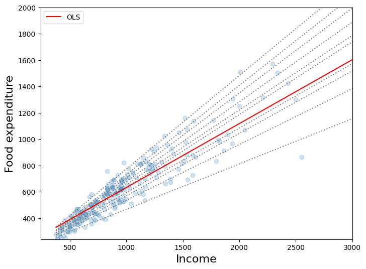
最初のプロット
このプロットは、10個の分位点回帰モデルの最良適合線と最小二乗法の適合線を比較しています。KoenkerとHallock(2001)が指摘しているように、以下が見られます。
食費は所得とともに増加する
食費の*分散*は所得とともに増加する
最小二乗法の推定値は、低所得の観測値に非常に適合が悪い(つまり、最小二乗法の直線がほとんどの低所得世帯を通過しない)
[5]:
x = np.arange(data.income.min(), data.income.max(), 50)
get_y = lambda a, b: a + b * x

fig, ax = plt.subplots(figsize=(8, 6))

for i in range(models.shape[0]):
    y = get_y(models.a[i], models.b[i])
    ax.plot(x, y, linestyle="dotted", color="grey")

y = get_y(ols["a"], ols["b"])

ax.plot(x, y, color="red", label="OLS")
ax.scatter(data.income, data.foodexp, alpha=0.2)
ax.set_xlim((240, 3000))
ax.set_ylim((240, 2000))
legend = ax.legend()
ax.set_xlabel("Income", fontsize=16)
ax.set_ylabel("Food expenditure", fontsize=16)
[5]:
Text(0, 0.5, 'Food expenditure')
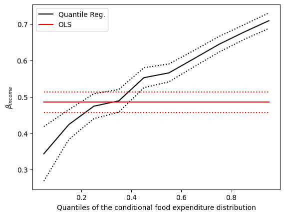
2番目のプロット
点線の黒線は、10個の分位点回帰推定値(実線の黒線)の周りの95%の点ごとの信頼区間を表しています。赤線は、最小二乗法回帰の結果とその95%信頼区間を表しています。
ほとんどの場合、分位点回帰の点推定値は最小二乗法の信頼区間外にあり、これは所得の食費支出への影響が分布全体で一定ではない可能性を示唆しています。
[6]:
n = models.shape[0]
p1 = plt.plot(models.q, models.b, color="black", label="Quantile Reg.")
p2 = plt.plot(models.q, models.ub, linestyle="dotted", color="black")
p3 = plt.plot(models.q, models.lb, linestyle="dotted", color="black")
p4 = plt.plot(models.q, [ols["b"]] * n, color="red", label="OLS")
p5 = plt.plot(models.q, [ols["lb"]] * n, linestyle="dotted", color="red")
p6 = plt.plot(models.q, [ols["ub"]] * n, linestyle="dotted", color="red")
plt.ylabel(r"$\beta_{income}$")
plt.xlabel("Quantiles of the conditional food expenditure distribution")
plt.legend()
plt.show()