再帰的最小二乗法
再帰的最小二乗法は、最小二乗法の拡張ウィンドウバージョンです。再帰的に計算された回帰係数が利用できることに加えて、再帰的に計算された残差は、パラメータの不安定性を調査するための統計量の構築に役立ちます。
RecursiveLS クラスでは、再帰的残差の計算と、CUSUMおよびCUSUM二乗統計量の計算が可能です。これらの統計量を、安定したパラメータという帰無仮説からの統計的に有意な偏差を示す基準線とともにプロットすることで、パラメータの安定性を視覚的に簡単に確認できます。
最後に、RecursiveLS モデルでは、パラメータベクトルに線形制約を課すことができ、式インターフェースを使用して構築できます。
[1]:
%matplotlib inline
import matplotlib.pyplot as plt
import numpy as np
import pandas as pd
import statsmodels.api as sm
from pandas_datareader.data import DataReader

np.set_printoptions(suppress=True)
例1:銅
最初に、銅データセット(下記の説明を参照)のパラメータの安定性を検討します。
[2]:
print(sm.datasets.copper.DESCRLONG)

dta = sm.datasets.copper.load_pandas().data
dta.index = pd.date_range("1951-01-01", "1975-01-01", freq="YS")
endog = dta["WORLDCONSUMPTION"]

# To the regressors in the dataset, we add a column of ones for an intercept
exog = sm.add_constant(
    dta[["COPPERPRICE", "INCOMEINDEX", "ALUMPRICE", "INVENTORYINDEX"]]
)
This data describes the world copper market from 1951 through 1975.  In an
example, in Gill, the outcome variable (of a 2 stage estimation) is the world
consumption of copper for the 25 years.  The explanatory variables are the
world consumption of copper in 1000 metric tons, the constant dollar adjusted
price of copper, the price of a substitute, aluminum, an index of real per
capita income base 1970, an annual measure of manufacturer inventory change,
and a time trend.
まず、モデルを構築して適合させ、サマリーを出力します。RLS モデルは回帰パラメータを再帰的に計算するため、データポイントと同じ数の推定値がありますが、サマリーテーブルにはサンプル全体で推定された回帰パラメータのみが表示されます。再帰の初期化による小さな影響を除けば、これらの推定値はOLS推定値と同等です。
[3]:
mod = sm.RecursiveLS(endog, exog)
res = mod.fit()

print(res.summary())
                           Statespace Model Results
==============================================================================
Dep. Variable:       WORLDCONSUMPTION   No. Observations:                   25
Model:                    RecursiveLS   Log Likelihood                -154.720
Date:                Thu, 03 Oct 2024   R-squared:                       0.965
Time:                        15:46:06   AIC                            319.441
Sample:                    01-01-1951   BIC                            325.535
                         - 01-01-1975   HQIC                           321.131
Covariance Type:            nonrobust   Scale                       117717.127
==================================================================================
                     coef    std err          z      P>|z|      [0.025      0.975]
----------------------------------------------------------------------------------
const          -6562.3719   2378.939     -2.759      0.006   -1.12e+04   -1899.737
COPPERPRICE      -13.8132     15.041     -0.918      0.358     -43.292      15.666
INCOMEINDEX      1.21e+04    763.401     15.853      0.000    1.06e+04    1.36e+04
ALUMPRICE         70.4146     32.678      2.155      0.031       6.367     134.462
INVENTORYINDEX   311.7330   2130.084      0.146      0.884   -3863.155    4486.621
===================================================================================
Ljung-Box (L1) (Q):                   2.17   Jarque-Bera (JB):                 1.70
Prob(Q):                              0.14   Prob(JB):                         0.43
Heteroskedasticity (H):               3.38   Skew:                            -0.67
Prob(H) (two-sided):                  0.13   Kurtosis:                         2.53
===================================================================================

Warnings:
[1] Parameters and covariance matrix estimates are RLS estimates conditional on the entire sample.
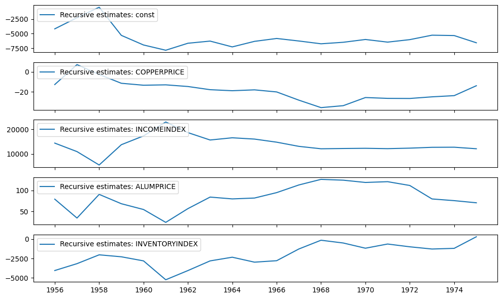
再帰係数は、recursive_coefficients 属性で利用できます。または、plot_recursive_coefficient メソッドを使用してプロットを生成できます。
[4]:
print(res.recursive_coefficients.filtered[0])
res.plot_recursive_coefficient(range(mod.k_exog), alpha=None, figsize=(10, 6))
[     2.88890087      4.94795049   1558.41803044   1958.43326658
 -51474.9578655   -4168.94974192  -2252.61351128   -446.55908507
  -5288.39794736  -6942.31935786  -7846.0890355   -6643.15121393
  -6274.11015558  -7272.01696292  -6319.02648554  -5822.23929148
  -6256.30902754  -6737.4044603   -6477.42841448  -5995.90746904
  -6450.80677813  -6022.92166487  -5258.35152753  -5320.89136363
  -6562.37193573]
[4]:

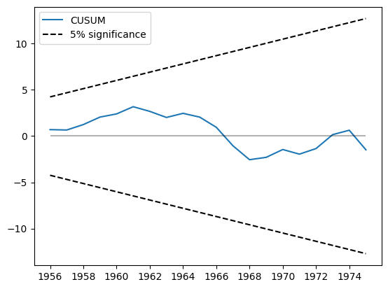
CUSUM統計量は cusum 属性で利用できますが、通常は plot_cusum メソッドを使用してパラメータの安定性を視覚的に確認する方が便利です。以下のプロットでは、CUSUM統計量は5%有意水準帯域外に移動しないため、5%水準で安定したパラメータという帰無仮説を棄却できません。
[5]:
print(res.cusum)
fig = res.plot_cusum()
[ 0.69971508  0.65841244  1.24629674  2.05476032  2.39888918  3.1786198
  2.67244672  2.01783215  2.46131747  2.05268638  0.95054336 -1.04505546
 -2.55465286 -2.29908152 -1.45289492 -1.95353993 -1.3504662   0.15789829
  0.6328653  -1.48184586]
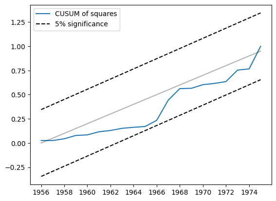
もう1つの関連する統計量は、CUSUM二乗です。cusum_squares 属性で利用できますが、同様に plot_cusum_squares メソッドを使用して視覚的に確認する方が便利です。以下のプロットでは、CUSUM二乗統計量は5%有意水準帯域外に移動しないため、5%水準で安定したパラメータという帰無仮説を棄却できません。
[6]:
res.plot_cusum_squares()
[6]:

例2:貨幣数量説
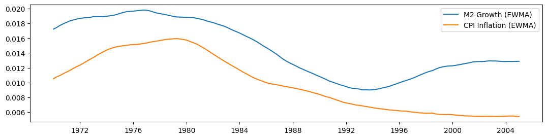
貨幣数量説は、「貨幣量の増加率の所定の変化は、…物価上昇率の同じ変化を誘発する」と示唆しています(Lucas、1980)。Lucasに倣い、貨幣増加率とCPIインフレ率の両側指数加重移動平均間の関係を調べます。Lucasはこれらの変数の関係が安定していることを発見しましたが、最近では関係が不安定になっているようです。例:Sargent and Surico(2010)を参照してください。
[7]:
start = "1959-12-01"
end = "2015-01-01"
m2 = DataReader("M2SL", "fred", start=start, end=end)
cpi = DataReader("CPIAUCSL", "fred", start=start, end=end)
[8]:
def ewma(series, beta, n_window):
    nobs = len(series)
    scalar = (1 - beta) / (1 + beta)
    ma = []
    k = np.arange(n_window, 0, -1)
    weights = np.r_[beta ** k, 1, beta ** k[::-1]]
    for t in range(n_window, nobs - n_window):
        window = series.iloc[t - n_window : t + n_window + 1].values
        ma.append(scalar * np.sum(weights * window))
    return pd.Series(ma, name=series.name, index=series.iloc[n_window:-n_window].index)


m2_ewma = ewma(np.log(m2["M2SL"].resample("QS").mean()).diff().iloc[1:], 0.95, 10 * 4)
cpi_ewma = ewma(
    np.log(cpi["CPIAUCSL"].resample("QS").mean()).diff().iloc[1:], 0.95, 10 * 4
)
Lucasの\(\beta = 0.95\)フィルター(両側に10年のウィンドウ)を使用して移動平均を構築した後、以下の各系列をプロットします。サンプルの一部では一緒に移動しているように見えますが、1990年以降は分岐しているように見えます。
[9]:
fig, ax = plt.subplots(figsize=(13, 3))

ax.plot(m2_ewma, label="M2 Growth (EWMA)")
ax.plot(cpi_ewma, label="CPI Inflation (EWMA)")
ax.legend()
[9]:
<matplotlib.legend.Legend at 0x7f6e8ca133a0>
[10]:
endog = cpi_ewma
exog = sm.add_constant(m2_ewma)
exog.columns = ["const", "M2"]

mod = sm.RecursiveLS(endog, exog)
res = mod.fit()

print(res.summary())
                           Statespace Model Results
==============================================================================
Dep. Variable:               CPIAUCSL   No. Observations:                  141
Model:                    RecursiveLS   Log Likelihood                 692.878
Date:                Thu, 03 Oct 2024   R-squared:                       0.813
Time:                        15:46:11   AIC                          -1381.755
Sample:                    01-01-1970   BIC                          -1375.858
                         - 01-01-2005   HQIC                         -1379.358
Covariance Type:            nonrobust   Scale                            0.000
==============================================================================
                 coef    std err          z      P>|z|      [0.025      0.975]
------------------------------------------------------------------------------
const         -0.0034      0.001     -6.013      0.000      -0.004      -0.002
M2             0.9128      0.037     24.601      0.000       0.840       0.986
===================================================================================
Ljung-Box (L1) (Q):                 138.23   Jarque-Bera (JB):                18.20
Prob(Q):                              0.00   Prob(JB):                         0.00
Heteroskedasticity (H):               5.30   Skew:                            -0.81
Prob(H) (two-sided):                  0.00   Kurtosis:                         2.27
===================================================================================

Warnings:
[1] Parameters and covariance matrix estimates are RLS estimates conditional on the entire sample.
[11]:
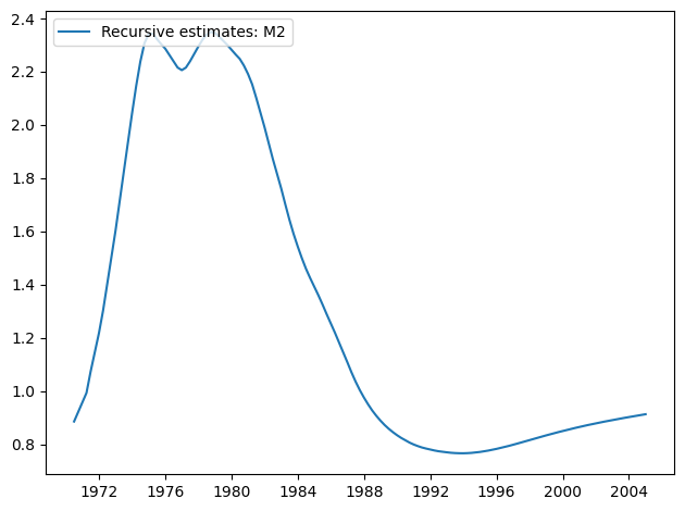
res.plot_recursive_coefficient(1, alpha=None)
[11]:

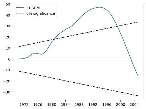
CUSUMプロットは、5%水準で大幅な偏差を示しており、パラメータの安定性という帰無仮説の棄却を示唆しています。
[12]:
res.plot_cusum()
[12]:

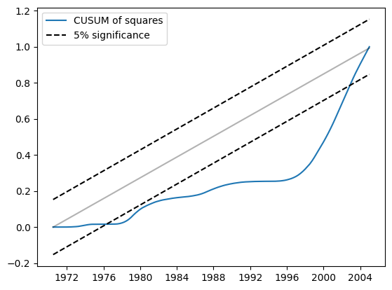
同様に、CUSUM二乗は5%水準で大幅な偏差を示しており、パラメータの安定性という帰無仮説の棄却も示唆しています。
[13]:
res.plot_cusum_squares()
[13]:

例3:線形制約と式
線形制約
モデルの構築時にconstraintsパラメータを使用することで、線形制約を実装することは難しくありません。
[14]:
endog = dta["WORLDCONSUMPTION"]
exog = sm.add_constant(
    dta[["COPPERPRICE", "INCOMEINDEX", "ALUMPRICE", "INVENTORYINDEX"]]
)

mod = sm.RecursiveLS(endog, exog, constraints="COPPERPRICE = ALUMPRICE")
res = mod.fit()
print(res.summary())
                           Statespace Model Results
==============================================================================
Dep. Variable:       WORLDCONSUMPTION   No. Observations:                   25
Model:                    RecursiveLS   Log Likelihood                -134.231
Date:                Thu, 03 Oct 2024   R-squared:                       0.989
Time:                        15:46:14   AIC                            276.462
Sample:                    01-01-1951   BIC                            281.338
                         - 01-01-1975   HQIC                           277.814
Covariance Type:            nonrobust   Scale                       137155.014
==================================================================================
                     coef    std err          z      P>|z|      [0.025      0.975]
----------------------------------------------------------------------------------
const          -4839.4836   2412.410     -2.006      0.045   -9567.721    -111.246
COPPERPRICE        5.9797     12.704      0.471      0.638     -18.921      30.880
INCOMEINDEX     1.115e+04    666.308     16.738      0.000    9847.000    1.25e+04
ALUMPRICE          5.9797     12.704      0.471      0.638     -18.921      30.880
INVENTORYINDEX   241.3452   2298.951      0.105      0.916   -4264.515    4747.206
===================================================================================
Ljung-Box (L1) (Q):                   6.27   Jarque-Bera (JB):                 1.78
Prob(Q):                              0.01   Prob(JB):                         0.41
Heteroskedasticity (H):               1.75   Skew:                            -0.63
Prob(H) (two-sided):                  0.48   Kurtosis:                         2.32
===================================================================================

Warnings:
[1] Parameters and covariance matrix estimates are RLS estimates conditional on the entire sample.
式
クラスメソッドfrom_formulaを使用して同じモデルを適合させることができます。
[15]:
mod = sm.RecursiveLS.from_formula(
    "WORLDCONSUMPTION ~ COPPERPRICE + INCOMEINDEX + ALUMPRICE + INVENTORYINDEX",
    dta,
    constraints="COPPERPRICE = ALUMPRICE",
)
res = mod.fit()
print(res.summary())
                           Statespace Model Results
==============================================================================
Dep. Variable:       WORLDCONSUMPTION   No. Observations:                   25
Model:                    RecursiveLS   Log Likelihood                -134.231
Date:                Thu, 03 Oct 2024   R-squared:                       0.989
Time:                        15:46:14   AIC                            276.462
Sample:                    01-01-1951   BIC                            281.338
                         - 01-01-1975   HQIC                           277.814
Covariance Type:            nonrobust   Scale                       137155.014
==================================================================================
                     coef    std err          z      P>|z|      [0.025      0.975]
----------------------------------------------------------------------------------
Intercept      -4839.4836   2412.410     -2.006      0.045   -9567.721    -111.246
COPPERPRICE        5.9797     12.704      0.471      0.638     -18.921      30.880
INCOMEINDEX     1.115e+04    666.308     16.738      0.000    9847.000    1.25e+04
ALUMPRICE          5.9797     12.704      0.471      0.638     -18.921      30.880
INVENTORYINDEX   241.3452   2298.951      0.105      0.916   -4264.515    4747.206
===================================================================================
Ljung-Box (L1) (Q):                   6.27   Jarque-Bera (JB):                 1.78
Prob(Q):                              0.01   Prob(JB):                         0.41
Heteroskedasticity (H):               1.75   Skew:                            -0.63
Prob(H) (two-sided):                  0.48   Kurtosis:                         2.32
===================================================================================

Warnings:
[1] Parameters and covariance matrix estimates are RLS estimates conditional on the entire sample.
/opt/hostedtoolcache/Python/3.10.15/x64/lib/python3.10/site-packages/statsmodels/tsa/base/tsa_model.py:473: ValueWarning: No frequency information was provided, so inferred frequency YS-JAN will be used.
  self._init_dates(dates, freq)