ローリング回帰
ローリングOLSは、固定された観測ウィンドウ全体にOLSを適用し、データセット全体でウィンドウをロール(移動またはスライド)します。重要なパラメータは、各OLS回帰で使用される観測数を決定する`window`です。デフォルトでは、`RollingOLS`はウィンドウ内の欠損値を削除するため、使用可能なデータポイントを使用してモデルを推定します。
推定値は、データポイント \(i+1, i+2, ... i+window\) を使用して推定されたモデルが位置 \(i+window\) に格納されるように調整されます。
このノートブックで使用されているモジュールをインポートすることから始めます。
[1]:
import matplotlib.pyplot as plt
import numpy as np
import pandas as pd
import pandas_datareader as pdr
import seaborn

import statsmodels.api as sm
from statsmodels.regression.rolling import RollingOLS

seaborn.set_style("darkgrid")
pd.plotting.register_matplotlib_converters()
%matplotlib inline
`pandas-datareader` は、Ken Frenchのウェブサイトからデータをダウンロードするために使用されます。ダウンロードされる2つのデータセットは、3つのFama-Frenchファクターと10の業界ポートフォリオです。データは1926年から入手できます。
データは、ファクターまたは業界ポートフォリオの月次リターンです。
[2]:
factors = pdr.get_data_famafrench("F-F_Research_Data_Factors", start="1-1-1926")[0]
factors.head()
/tmp/ipykernel_3995/1924419770.py:1: FutureWarning: The argument 'date_parser' is deprecated and will be removed in a future version. Please use 'date_format' instead, or read your data in as 'object' dtype and then call 'to_datetime'.
  factors = pdr.get_data_famafrench("F-F_Research_Data_Factors", start="1-1-1926")[0]
[2]:
| Mkt-RF (市場超過収益率) | SMB (規模ファクター) | HML (バリューファクター) | RF (リスクフリーレート) | |
|---|---|---|---|---|
| Date (日付) | ||||
| 1926-07 | 2.96 | -2.56 | -2.43 | 0.22 |
| 1926-08 | 2.64 | -1.17 | 3.82 | 0.25 |
| 1926-09 | 0.36 | -1.40 | 0.13 | 0.23 |
| 1926-10 | -3.24 | -0.09 | 0.70 | 0.32 |
| 1926-11 | 2.53 | -0.10 | -0.51 | 0.31 |
[3]:
industries = pdr.get_data_famafrench("10_Industry_Portfolios", start="1-1-1926")[0]
industries.head()
/tmp/ipykernel_3995/268191425.py:1: FutureWarning: The argument 'date_parser' is deprecated and will be removed in a future version. Please use 'date_format' instead, or read your data in as 'object' dtype and then call 'to_datetime'.
  industries = pdr.get_data_famafrench("10_Industry_Portfolios", start="1-1-1926")[0]
[3]:
| NoDur (非耐久消費財) | Durbl (耐久消費財) | Manuf (製造業) | Enrgy (エネルギー) | HiTec (ハイテク) | Telcm (通信) | Shops (小売) | Hlth (ヘルスケア) | Utils (公益事業) | Other (その他) | |
|---|---|---|---|---|---|---|---|---|---|---|
| Date (日付) | ||||||||||
| 1926-07 | 1.45 | 15.55 | 4.69 | -1.18 | 2.90 | 0.83 | 0.11 | 1.77 | 7.04 | 2.13 |
| 1926-08 | 3.97 | 3.68 | 2.81 | 3.47 | 2.66 | 2.17 | -0.71 | 4.25 | -1.69 | 4.35 |
| 1926-09 | 1.14 | 4.80 | 1.15 | -3.39 | -0.38 | 2.41 | 0.21 | 0.69 | 2.04 | 0.29 |
| 1926-10 | -1.24 | -8.23 | -3.63 | -0.78 | -4.58 | -0.11 | -2.29 | -0.57 | -2.63 | -2.84 |
| 1926-11 | 5.20 | -0.19 | 4.10 | 0.01 | 4.71 | 1.63 | 6.43 | 5.42 | 3.71 | 2.11 |
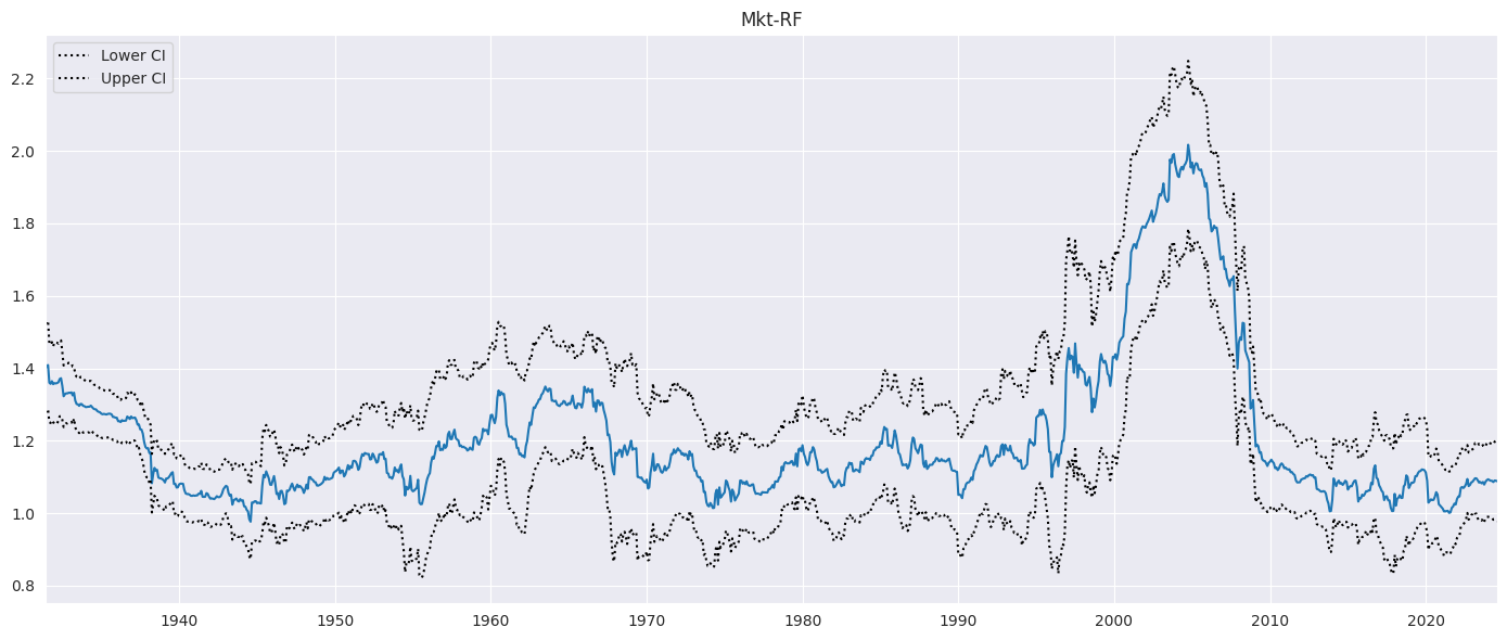
最初に推定されるモデルは、テクノロジーセクター企業の超過収益率を市場の超過収益率に回帰させるCAPMのローリングバージョンです。
ウィンドウは60か月であるため、最初の60 (`window`)か月後に結果が得られます。最初の59 (`window` - 1)個の推定値はすべて`nan`で埋められます。
[4]:
endog = industries.HiTec - factors.RF.values
exog = sm.add_constant(factors["Mkt-RF"])
rols = RollingOLS(endog, exog, window=60)
rres = rols.fit()
params = rres.params.copy()
params.index = np.arange(1, params.shape[0] + 1)
params.head()
[4]:
| const (定数項) | Mkt-RF (市場超過収益率) | |
|---|---|---|
| 1 | NaN (欠損値) | NaN (欠損値) |
| 2 | NaN (欠損値) | NaN (欠損値) |
| 3 | NaN (欠損値) | NaN (欠損値) |
| 4 | NaN (欠損値) | NaN (欠損値) |
| 5 | NaN (欠損値) | NaN (欠損値) |
[5]:
params.iloc[57:62]
[5]:
| const (定数項) | Mkt-RF (市場超過収益率) | |
|---|---|---|
| 58 | NaN (欠損値) | NaN (欠損値) |
| 59 | NaN (欠損値) | NaN (欠損値) |
| 60 | 0.876155 | 1.399240 |
| 61 | 0.879936 | 1.406578 |
| 62 | 0.953169 | 1.408826 |
[6]:
params.tail()
[6]:
| const (定数項) | Mkt-RF (市場超過収益率) | |
|---|---|---|
| 1174 | 0.480235 | 1.089338 |
| 1175 | 0.552565 | 1.086061 |
| 1176 | 0.610923 | 1.090145 |
| 1177 | 0.517339 | 1.089693 |
| 1178 | 0.503159 | 1.088327 |
次に、市場のベータ値を95%の点ごとの信頼区間とともにプロットします。 `alpha=False` は、存在する場合、定数項の列を省略します。
[7]:
fig = rres.plot_recursive_coefficient(variables=["Mkt-RF"], figsize=(14, 6))
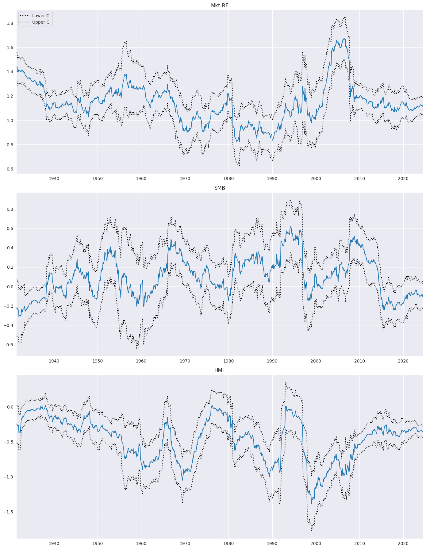
次に、モデルを拡張して、3つのファクターすべて(市場超過収益率、規模ファクター、バリューファクター)を含めます。
[8]:
exog_vars = ["Mkt-RF", "SMB", "HML"]
exog = sm.add_constant(factors[exog_vars])
rols = RollingOLS(endog, exog, window=60)
rres = rols.fit()
fig = rres.plot_recursive_coefficient(variables=exog_vars, figsize=(14, 18))
式
`RollingOLS` と `RollingWLS` はどちらも、式インターフェースを使用したモデル指定をサポートしています。以下の例は、以前に推定された3ファクターモデルと同等です。有効なPython変数名を持つように、1つの変数の名前が変更されていることに注意してください。
[9]:
joined = pd.concat([factors, industries], axis=1)
joined["Mkt_RF"] = joined["Mkt-RF"]
mod = RollingOLS.from_formula("HiTec ~ Mkt_RF + SMB + HML", data=joined, window=60)
rres = mod.fit()
rres.params.tail()
[9]:
| Intercept (切片) | Mkt_RF (市場超過収益率) | SMB (規模ファクター) | HML (バリューファクター) | |
|---|---|---|---|---|
| Date (日付) | ||||
| 2024-04 | 0.600109 | 1.121680 | -0.095098 | -0.344825 |
| 2024-05 | 0.682975 | 1.114558 | -0.091375 | -0.351516 |
| 2024-06 | 0.719744 | 1.121549 | -0.106960 | -0.357406 |
| 2024-07 | 0.674874 | 1.122952 | -0.115250 | -0.361814 |
| 2024-08 | 0.691445 | 1.116360 | -0.108656 | -0.368933 |
`RollingWLS`: ローリング加重最小二乗法
`rolling` モジュールは、ローリング加重最小二乗法を実行するためのオプションの `weights` 入力を取る `RollingWLS` も提供します。これは、ローリングデータウィンドウに適用した場合に `WLS` と一致する結果を生成します。
フィットオプション
Fitは、共分散推定量を設定するための他のオプションのキーワードを受け入れます。サポートされている推定量は、`nonrobust`(従来のOLS推定量)と `HC0`(Whiteの異分散性堅牢推定量)の2つだけです。
モデルパラメータのみを推定するために、`params_only=True` を設定できます。これは、推論を実行するために必要な値のフルセットを計算するよりも大幅に高速です。
最後に、パラメータ `reset` を正の整数に設定して、非常に長いサンプルの推定誤差を制御できます。 `RollingOLS` は、ローリング時に最新の観測値のみを追加し、サンプルをロールするときに削除された観測値を削除することにより、完全な行列積を回避します。 `reset` を設定すると、`reset` 周期ごとに完全な内積が使用されます。ほとんどのアプリケーションでは、このパラメータは省略できます。
[10]:
%timeit rols.fit()
%timeit rols.fit(params_only=True)
321 ms ± 30.9 ms per loop (mean ± std. dev. of 7 runs, 1 loop each)
69.8 ms ± 8.5 ms per loop (mean ± std. dev. of 7 runs, 10 loops each)
サンプルの拡張
ウィンドウ全体の長さに十分な観測値が得られるまで、サンプルを拡張することができます。この例では、12個の観測値が利用可能になったら開始し、60個の観測値が利用可能になるまでサンプルを増やします。最初の非 `nan` 値は12個の観測値を使用して計算され、2番目は13個の観測値を使用して計算されます。他のすべての推定値は60個の観測値を使用して計算されます。
[11]:
res = RollingOLS(endog, exog, window=60, min_nobs=12, expanding=True).fit()
res.params.iloc[10:15]
[11]:
| const (定数項) | Mkt-RF (市場超過収益率) | SMB (規模ファクター) | HML (バリューファクター) | |
|---|---|---|---|---|
| Date (日付) | ||||
| 1927-05 | NaN (欠損値) | NaN (欠損値) | NaN (欠損値) | NaN (欠損値) |
| 1927-06 | 1.560283 | 0.999383 | 1.351219 | -0.471879 |
| 1927-07 | 1.235899 | 1.294857 | 0.742924 | -0.540048 |
| 1927-08 | 1.249999 | 1.297546 | 0.752327 | -0.548306 |
| 1927-09 | 1.375626 | 1.286724 | 1.177758 | -0.609331 |
[12]:
res.nobs[10:15]
[12]:
Date
1927-05     0
1927-06    12
1927-07    13
1927-08    14
1927-09    15
Freq: M, dtype: int64