時系列モデルにおける決定論的項
[1]:
import matplotlib.pyplot as plt
import numpy as np
import pandas as pd

plt.rc("figure", figsize=(16, 9))
plt.rc("font", size=16)
基本的な使用方法
基本的な設定は、DeterministicProcessを通して直接構築できます。これらには、定数、任意の次数を持つ時間トレンド、季節成分またはフーリエ成分が含まれます。
このプロセスには、完全サンプル(またはサンプル内)のインデックスが必要です。
まず、定数、線形時間トレンド、5期間の季節項を持つ決定論的プロセスを初期化します。in_sampleメソッドは、インデックスに一致する値の完全なセットを返します。
[2]:
from statsmodels.tsa.deterministic import DeterministicProcess

index = pd.RangeIndex(0, 100)
det_proc = DeterministicProcess(index, constant=True, order=1, seasonal=True, period=5)
det_proc.in_sample()
[2]:
| 定数 | トレンド | s(2,5) | s(3,5) | s(4,5) | s(5,5) | |
|---|---|---|---|---|---|---|
| 0 | 1.0 | 1.0 | 0.0 | 0.0 | 0.0 | 0.0 |
| 1 | 1.0 | 2.0 | 1.0 | 0.0 | 0.0 | 0.0 |
| 2 | 1.0 | 3.0 | 0.0 | 1.0 | 0.0 | 0.0 |
| 3 | 1.0 | 4.0 | 0.0 | 0.0 | 1.0 | 0.0 |
| 4 | 1.0 | 5.0 | 0.0 | 0.0 | 0.0 | 1.0 |
| ... | ... | ... | ... | ... | ... | ... |
| 95 | 1.0 | 96.0 | 0.0 | 0.0 | 0.0 | 0.0 |
| 96 | 1.0 | 97.0 | 1.0 | 0.0 | 0.0 | 0.0 |
| 97 | 1.0 | 98.0 | 0.0 | 1.0 | 0.0 | 0.0 |
| 98 | 1.0 | 99.0 | 0.0 | 0.0 | 1.0 | 0.0 |
| 99 | 1.0 | 100.0 | 0.0 | 0.0 | 0.0 | 1.0 |
100行×6列
out_of_sampleは、サンプルの終了後に続くsteps個の値を返します。
[3]:
det_proc.out_of_sample(15)
[3]:
| 定数 | トレンド | s(2,5) | s(3,5) | s(4,5) | s(5,5) | |
|---|---|---|---|---|---|---|
| 100 | 1.0 | 101.0 | 0.0 | 0.0 | 0.0 | 0.0 |
| 101 | 1.0 | 102.0 | 1.0 | 0.0 | 0.0 | 0.0 |
| 102 | 1.0 | 103.0 | 0.0 | 1.0 | 0.0 | 0.0 |
| 103 | 1.0 | 104.0 | 0.0 | 0.0 | 1.0 | 0.0 |
| 104 | 1.0 | 105.0 | 0.0 | 0.0 | 0.0 | 1.0 |
| 105 | 1.0 | 106.0 | 0.0 | 0.0 | 0.0 | 0.0 |
| 106 | 1.0 | 107.0 | 1.0 | 0.0 | 0.0 | 0.0 |
| 107 | 1.0 | 108.0 | 0.0 | 1.0 | 0.0 | 0.0 |
| 108 | 1.0 | 109.0 | 0.0 | 0.0 | 1.0 | 0.0 |
| 109 | 1.0 | 110.0 | 0.0 | 0.0 | 0.0 | 1.0 |
| 110 | 1.0 | 111.0 | 0.0 | 0.0 | 0.0 | 0.0 |
| 111 | 1.0 | 112.0 | 1.0 | 0.0 | 0.0 | 0.0 |
| 112 | 1.0 | 113.0 | 0.0 | 1.0 | 0.0 | 0.0 |
| 113 | 1.0 | 114.0 | 0.0 | 0.0 | 1.0 | 0.0 |
| 114 | 1.0 | 115.0 | 0.0 | 0.0 | 0.0 | 1.0 |
range(start, stop)も、サンプル内とサンプル外の範囲を含む任意の範囲で決定論的項を生成するために使用できます。
備考
インデックスがpandasの
DatetimeIndexまたはPeriodIndexの場合、startとstopは日付のような値(文字列、例:「2020-06-01」、またはTimestamp)または整数にすることができます。stopは常に範囲に含まれます。これはPythonicではないですが、statsmodelsとPandasの両方が日付のようなスライスを扱う際にstopを含める必要があるためです。
[4]:
det_proc.range(190, 210)
[4]:
| 定数 | トレンド | s(2,5) | s(3,5) | s(4,5) | s(5,5) | |
|---|---|---|---|---|---|---|
| 190 | 1.0 | 191.0 | 0.0 | 0.0 | 0.0 | 0.0 |
| 191 | 1.0 | 192.0 | 1.0 | 0.0 | 0.0 | 0.0 |
| 192 | 1.0 | 193.0 | 0.0 | 1.0 | 0.0 | 0.0 |
| 193 | 1.0 | 194.0 | 0.0 | 0.0 | 1.0 | 0.0 |
| 194 | 1.0 | 195.0 | 0.0 | 0.0 | 0.0 | 1.0 |
| 195 | 1.0 | 196.0 | 0.0 | 0.0 | 0.0 | 0.0 |
| 196 | 1.0 | 197.0 | 1.0 | 0.0 | 0.0 | 0.0 |
| 197 | 1.0 | 198.0 | 0.0 | 1.0 | 0.0 | 0.0 |
| 198 | 1.0 | 199.0 | 0.0 | 0.0 | 1.0 | 0.0 |
| 199 | 1.0 | 200.0 | 0.0 | 0.0 | 0.0 | 1.0 |
| 200 | 1.0 | 201.0 | 0.0 | 0.0 | 0.0 | 0.0 |
| 201 | 1.0 | 202.0 | 1.0 | 0.0 | 0.0 | 0.0 |
| 202 | 1.0 | 203.0 | 0.0 | 1.0 | 0.0 | 0.0 |
| 203 | 1.0 | 204.0 | 0.0 | 0.0 | 1.0 | 0.0 |
| 204 | 1.0 | 205.0 | 0.0 | 0.0 | 0.0 | 1.0 |
| 205 | 1.0 | 206.0 | 0.0 | 0.0 | 0.0 | 0.0 |
| 206 | 1.0 | 207.0 | 1.0 | 0.0 | 0.0 | 0.0 |
| 207 | 1.0 | 208.0 | 0.0 | 1.0 | 0.0 | 0.0 |
| 208 | 1.0 | 209.0 | 0.0 | 0.0 | 1.0 | 0.0 |
| 209 | 1.0 | 210.0 | 0.0 | 0.0 | 0.0 | 1.0 |
| 210 | 1.0 | 211.0 | 0.0 | 0.0 | 0.0 | 0.0 |
日付のようなインデックスの使用
次に、PeriodIndexを使用して同じ手順を示します。
[5]:
index = pd.period_range("2020-03-01", freq="M", periods=60)
det_proc = DeterministicProcess(index, constant=True, fourier=2)
det_proc.in_sample().head(12)
[5]:
| 定数 | sin(1,12) | cos(1,12) | sin(2,12) | cos(2,12) | |
|---|---|---|---|---|---|
| 2020-03 | 1.0 | 0.000000e+00 | 1.000000e+00 | 0.000000e+00 | 1.0 |
| 2020-04 | 1.0 | 5.000000e-01 | 8.660254e-01 | 8.660254e-01 | 0.5 |
| 2020-05 | 1.0 | 8.660254e-01 | 5.000000e-01 | 8.660254e-01 | -0.5 |
| 2020-06 | 1.0 | 1.000000e+00 | 6.123234e-17 | 1.224647e-16 | -1.0 |
| 2020-07 | 1.0 | 8.660254e-01 | -5.000000e-01 | -8.660254e-01 | -0.5 |
| 2020-08 | 1.0 | 5.000000e-01 | -8.660254e-01 | -8.660254e-01 | 0.5 |
| 2020-09 | 1.0 | 1.224647e-16 | -1.000000e+00 | -2.449294e-16 | 1.0 |
| 2020-10 | 1.0 | -5.000000e-01 | -8.660254e-01 | 8.660254e-01 | 0.5 |
| 2020-11 | 1.0 | -8.660254e-01 | -5.000000e-01 | 8.660254e-01 | -0.5 |
| 2020-12 | 1.0 | -1.000000e+00 | -1.836970e-16 | 3.673940e-16 | -1.0 |
| 2021-01 | 1.0 | -8.660254e-01 | 5.000000e-01 | -8.660254e-01 | -0.5 |
| 2021-02 | 1.0 | -5.000000e-01 | 8.660254e-01 | -8.660254e-01 | 0.5 |
[6]:
det_proc.out_of_sample(12)
[6]:
| 定数 | sin(1,12) | cos(1,12) | sin(2,12) | cos(2,12) | |
|---|---|---|---|---|---|
| 2025-03 | 1.0 | -1.224647e-15 | 1.000000e+00 | -2.449294e-15 | 1.0 |
| 2025-04 | 1.0 | 5.000000e-01 | 8.660254e-01 | 8.660254e-01 | 0.5 |
| 2025-05 | 1.0 | 8.660254e-01 | 5.000000e-01 | 8.660254e-01 | -0.5 |
| 2025-06 | 1.0 | 1.000000e+00 | -4.904777e-16 | -9.809554e-16 | -1.0 |
| 2025-07 | 1.0 | 8.660254e-01 | -5.000000e-01 | -8.660254e-01 | -0.5 |
| 2025-08 | 1.0 | 5.000000e-01 | -8.660254e-01 | -8.660254e-01 | 0.5 |
| 2025-09 | 1.0 | 4.899825e-15 | -1.000000e+00 | -9.799650e-15 | 1.0 |
| 2025-10 | 1.0 | -5.000000e-01 | -8.660254e-01 | 8.660254e-01 | 0.5 |
| 2025-11 | 1.0 | -8.660254e-01 | -5.000000e-01 | 8.660254e-01 | -0.5 |
| 2025-12 | 1.0 | -1.000000e+00 | -3.184701e-15 | 6.369401e-15 | -1.0 |
| 2026-01 | 1.0 | -8.660254e-01 | 5.000000e-01 | -8.660254e-01 | -0.5 |
| 2026-02 | 1.0 | -5.000000e-01 | 8.660254e-01 | -8.660254e-01 | 0.5 |
rangeは日付のような引数を受け入れます。これは通常、文字列として与えられます。
[7]:
det_proc.range("2025-01", "2026-01")
[7]:
| 定数 | sin(1,12) | cos(1,12) | sin(2,12) | cos(2,12) | |
|---|---|---|---|---|---|
| 2025-01 | 1.0 | -8.660254e-01 | 5.000000e-01 | -8.660254e-01 | -0.5 |
| 2025-02 | 1.0 | -5.000000e-01 | 8.660254e-01 | -8.660254e-01 | 0.5 |
| 2025-03 | 1.0 | -1.224647e-15 | 1.000000e+00 | -2.449294e-15 | 1.0 |
| 2025-04 | 1.0 | 5.000000e-01 | 8.660254e-01 | 8.660254e-01 | 0.5 |
| 2025-05 | 1.0 | 8.660254e-01 | 5.000000e-01 | 8.660254e-01 | -0.5 |
| 2025-06 | 1.0 | 1.000000e+00 | -4.904777e-16 | -9.809554e-16 | -1.0 |
| 2025-07 | 1.0 | 8.660254e-01 | -5.000000e-01 | -8.660254e-01 | -0.5 |
| 2025-08 | 1.0 | 5.000000e-01 | -8.660254e-01 | -8.660254e-01 | 0.5 |
| 2025-09 | 1.0 | 4.899825e-15 | -1.000000e+00 | -9.799650e-15 | 1.0 |
| 2025-10 | 1.0 | -5.000000e-01 | -8.660254e-01 | 8.660254e-01 | 0.5 |
| 2025-11 | 1.0 | -8.660254e-01 | -5.000000e-01 | 8.660254e-01 | -0.5 |
| 2025-12 | 1.0 | -1.000000e+00 | -3.184701e-15 | 6.369401e-15 | -1.0 |
| 2026-01 | 1.0 | -8.660254e-01 | 5.000000e-01 | -8.660254e-01 | -0.5 |
これは、整数値58と70を使用することと同じです。
[8]:
det_proc.range(58, 70)
[8]:
| 定数 | sin(1,12) | cos(1,12) | sin(2,12) | cos(2,12) | |
|---|---|---|---|---|---|
| 2025-01 | 1.0 | -8.660254e-01 | 5.000000e-01 | -8.660254e-01 | -0.5 |
| 2025-02 | 1.0 | -5.000000e-01 | 8.660254e-01 | -8.660254e-01 | 0.5 |
| 2025-03 | 1.0 | -1.224647e-15 | 1.000000e+00 | -2.449294e-15 | 1.0 |
| 2025-04 | 1.0 | 5.000000e-01 | 8.660254e-01 | 8.660254e-01 | 0.5 |
| 2025-05 | 1.0 | 8.660254e-01 | 5.000000e-01 | 8.660254e-01 | -0.5 |
| 2025-06 | 1.0 | 1.000000e+00 | -4.904777e-16 | -9.809554e-16 | -1.0 |
| 2025-07 | 1.0 | 8.660254e-01 | -5.000000e-01 | -8.660254e-01 | -0.5 |
| 2025-08 | 1.0 | 5.000000e-01 | -8.660254e-01 | -8.660254e-01 | 0.5 |
| 2025-09 | 1.0 | 4.899825e-15 | -1.000000e+00 | -9.799650e-15 | 1.0 |
| 2025-10 | 1.0 | -5.000000e-01 | -8.660254e-01 | 8.660254e-01 | 0.5 |
| 2025-11 | 1.0 | -8.660254e-01 | -5.000000e-01 | 8.660254e-01 | -0.5 |
| 2025-12 | 1.0 | -1.000000e+00 | -3.184701e-15 | 6.369401e-15 | -1.0 |
| 2026-01 | 1.0 | -8.660254e-01 | 5.000000e-01 | -8.660254e-01 | -0.5 |
高度な構築
コンストラクタでは直接サポートされていない機能を持つ決定論的プロセスは、DetermisticTermのリストを受け入れるadditional_termsを使用して作成できます。ここでは、2つの季節成分を持つ決定論的プロセスを作成します。1つは5日周期の曜日、もう1つは365.25日周期のフーリエ成分によって捉えられる年間成分です。
[9]:
from statsmodels.tsa.deterministic import Fourier, Seasonality, TimeTrend

index = pd.period_range("2020-03-01", freq="D", periods=2 * 365)
tt = TimeTrend(constant=True)
four = Fourier(period=365.25, order=2)
seas = Seasonality(period=7)
det_proc = DeterministicProcess(index, additional_terms=[tt, seas, four])
det_proc.in_sample().head(28)
[9]:
| 定数 | s(2,7) | s(3,7) | s(4,7) | s(5,7) | s(6,7) | s(7,7) | sin(1,365.25) | cos(1,365.25) | sin(2,365.25) | cos(2,365.25) | |
|---|---|---|---|---|---|---|---|---|---|---|---|
| 2020-03-01 | 1.0 | 0.0 | 0.0 | 0.0 | 0.0 | 0.0 | 0.0 | 0.000000 | 1.000000 | 0.000000 | 1.000000 |
| 2020-03-02 | 1.0 | 1.0 | 0.0 | 0.0 | 0.0 | 0.0 | 0.0 | 0.017202 | 0.999852 | 0.034398 | 0.999408 |
| 2020-03-03 | 1.0 | 0.0 | 1.0 | 0.0 | 0.0 | 0.0 | 0.0 | 0.034398 | 0.999408 | 0.068755 | 0.997634 |
| 2020-03-04 | 1.0 | 0.0 | 0.0 | 1.0 | 0.0 | 0.0 | 0.0 | 0.051584 | 0.998669 | 0.103031 | 0.994678 |
| 2020-03-05 | 1.0 | 0.0 | 0.0 | 0.0 | 1.0 | 0.0 | 0.0 | 0.068755 | 0.997634 | 0.137185 | 0.990545 |
| 2020-03-06 | 1.0 | 0.0 | 0.0 | 0.0 | 0.0 | 1.0 | 0.0 | 0.085906 | 0.996303 | 0.171177 | 0.985240 |
| 2020-03-07 | 1.0 | 0.0 | 0.0 | 0.0 | 0.0 | 0.0 | 1.0 | 0.103031 | 0.994678 | 0.204966 | 0.978769 |
| 2020-03-08 | 1.0 | 0.0 | 0.0 | 0.0 | 0.0 | 0.0 | 0.0 | 0.120126 | 0.992759 | 0.238513 | 0.971139 |
| 2020-03-09 | 1.0 | 1.0 | 0.0 | 0.0 | 0.0 | 0.0 | 0.0 | 0.137185 | 0.990545 | 0.271777 | 0.962360 |
| 2020-03-10 | 1.0 | 0.0 | 1.0 | 0.0 | 0.0 | 0.0 | 0.0 | 0.154204 | 0.988039 | 0.304719 | 0.952442 |
| 2020-03-11 | 1.0 | 0.0 | 0.0 | 1.0 | 0.0 | 0.0 | 0.0 | 0.171177 | 0.985240 | 0.337301 | 0.941397 |
| 2020-03-12 | 1.0 | 0.0 | 0.0 | 0.0 | 1.0 | 0.0 | 0.0 | 0.188099 | 0.982150 | 0.369484 | 0.929237 |
| 2020-03-13 | 1.0 | 0.0 | 0.0 | 0.0 | 0.0 | 1.0 | 0.0 | 0.204966 | 0.978769 | 0.401229 | 0.915978 |
| 2020-03-14 | 1.0 | 0.0 | 0.0 | 0.0 | 0.0 | 0.0 | 1.0 | 0.221772 | 0.975099 | 0.432499 | 0.901634 |
| 2020-03-15 | 1.0 | 0.0 | 0.0 | 0.0 | 0.0 | 0.0 | 0.0 | 0.238513 | 0.971139 | 0.463258 | 0.886224 |
| 2020-03-16 | 1.0 | 1.0 | 0.0 | 0.0 | 0.0 | 0.0 | 0.0 | 0.255182 | 0.966893 | 0.493468 | 0.869764 |
| 2020-03-17 | 1.0 | 0.0 | 1.0 | 0.0 | 0.0 | 0.0 | 0.0 | 0.271777 | 0.962360 | 0.523094 | 0.852275 |
| 2020-03-18 | 1.0 | 0.0 | 0.0 | 1.0 | 0.0 | 0.0 | 0.0 | 0.288291 | 0.957543 | 0.552101 | 0.833777 |
| 2020-03-19 | 1.0 | 0.0 | 0.0 | 0.0 | 1.0 | 0.0 | 0.0 | 0.304719 | 0.952442 | 0.580455 | 0.814292 |
| 2020-03-20 | 1.0 | 0.0 | 0.0 | 0.0 | 0.0 | 1.0 | 0.0 | 0.321058 | 0.947060 | 0.608121 | 0.793844 |
| 2020-03-21 | 1.0 | 0.0 | 0.0 | 0.0 | 0.0 | 0.0 | 1.0 | 0.337301 | 0.941397 | 0.635068 | 0.772456 |
| 2020-03-22 | 1.0 | 0.0 | 0.0 | 0.0 | 0.0 | 0.0 | 0.0 | 0.353445 | 0.935455 | 0.661263 | 0.750154 |
| 2020-03-23 | 1.0 | 1.0 | 0.0 | 0.0 | 0.0 | 0.0 | 0.0 | 0.369484 | 0.929237 | 0.686676 | 0.726964 |
| 2020-03-24 | 1.0 | 0.0 | 1.0 | 0.0 | 0.0 | 0.0 | 0.0 | 0.385413 | 0.922744 | 0.711276 | 0.702913 |
| 2020-03-25 | 1.0 | 0.0 | 0.0 | 1.0 | 0.0 | 0.0 | 0.0 | 0.401229 | 0.915978 | 0.735034 | 0.678031 |
| 2020-03-26 | 1.0 | 0.0 | 0.0 | 0.0 | 1.0 | 0.0 | 0.0 | 0.416926 | 0.908940 | 0.757922 | 0.652346 |
| 2020-03-27 | 1.0 | 0.0 | 0.0 | 0.0 | 0.0 | 1.0 | 0.0 | 0.432499 | 0.901634 | 0.779913 | 0.625889 |
| 2020-03-28 | 1.0 | 0.0 | 0.0 | 0.0 | 0.0 | 0.0 | 1.0 | 0.447945 | 0.894061 | 0.800980 | 0.598691 |
カスタム決定論的項
DetermisticTerm抽象基本クラスは、ユーザーがカスタム決定論的項を作成するためのサブクラス化を目的として設計されています。次に2つの例を示します。1つ目は、一定期間後にブレークを許容するブロークンタイムトレンドです。2つ目は、「トリック」決定論的項であり、外生データ(これは実際には決定論的プロセスではありません)を決定論的であるかのように扱うことができます。これにより、予測に必要な項の収集を簡素化できます。
これらは、カスタム項の構築を示すことを目的としています。入力検証の観点から、間違いなく改善できます。
[10]:
from statsmodels.tsa.deterministic import DeterministicTerm


class BrokenTimeTrend(DeterministicTerm):
    def __init__(self, break_period: int):
        self._break_period = break_period

    def __str__(self):
        return "Broken Time Trend"

    def _eq_attr(self):
        return (self._break_period,)

    def in_sample(self, index: pd.Index):
        nobs = index.shape[0]
        terms = np.zeros((nobs, 2))
        terms[self._break_period :, 0] = 1
        terms[self._break_period :, 1] = np.arange(self._break_period + 1, nobs + 1)
        return pd.DataFrame(terms, columns=["const_break", "trend_break"], index=index)

    def out_of_sample(
        self, steps: int, index: pd.Index, forecast_index: pd.Index = None
    ):
        # Always call extend index first
        fcast_index = self._extend_index(index, steps, forecast_index)
        nobs = index.shape[0]
        terms = np.zeros((steps, 2))
        # Assume break period is in-sample
        terms[:, 0] = 1
        terms[:, 1] = np.arange(nobs + 1, nobs + steps + 1)
        return pd.DataFrame(
            terms, columns=["const_break", "trend_break"], index=fcast_index
        )
[11]:
btt = BrokenTimeTrend(60)
tt = TimeTrend(constant=True, order=1)
index = pd.RangeIndex(100)
det_proc = DeterministicProcess(index, additional_terms=[tt, btt])
det_proc.range(55, 65)
[11]:
| 定数 | トレンド | const_break | trend_break | |
|---|---|---|---|---|
| 55 | 1.0 | 56.0 | 0.0 | 0.0 |
| 56 | 1.0 | 57.0 | 0.0 | 0.0 |
| 57 | 1.0 | 58.0 | 0.0 | 0.0 |
| 58 | 1.0 | 59.0 | 0.0 | 0.0 |
| 59 | 1.0 | 60.0 | 0.0 | 0.0 |
| 60 | 1.0 | 61.0 | 1.0 | 61.0 |
| 61 | 1.0 | 62.0 | 1.0 | 62.0 |
| 62 | 1.0 | 63.0 | 1.0 | 63.0 |
| 63 | 1.0 | 64.0 | 1.0 | 64.0 |
| 64 | 1.0 | 65.0 | 1.0 | 65.0 |
| 65 | 1.0 | 66.0 | 1.0 | 66.0 |
次に、予測のためのサンプル外の外生配列の構築を簡素化する、実際の外生データの単純な「ラッパー」を作成します。
[12]:
class ExogenousProcess(DeterministicTerm):
    def __init__(self, data):
        self._data = data

    def __str__(self):
        return "Custom Exog Process"

    def _eq_attr(self):
        return (id(self._data),)

    def in_sample(self, index: pd.Index):
        return self._data.loc[index]

    def out_of_sample(
        self, steps: int, index: pd.Index, forecast_index: pd.Index = None
    ):
        forecast_index = self._extend_index(index, steps, forecast_index)
        return self._data.loc[forecast_index]
[13]:
import numpy as np

gen = np.random.default_rng(98765432101234567890)
exog = pd.DataFrame(gen.integers(100, size=(300, 2)), columns=["exog1", "exog2"])
exog.head()
[13]:
| exog1 | exog2 | |
|---|---|---|
| 0 | 6 | 99 |
| 1 | 64 | 28 |
| 2 | 15 | 81 |
| 3 | 54 | 8 |
| 4 | 12 | 8 |
[14]:
ep = ExogenousProcess(exog)
tt = TimeTrend(constant=True, order=1)
# The in-sample index
idx = exog.index[:200]
det_proc = DeterministicProcess(idx, additional_terms=[tt, ep])
[15]:
det_proc.in_sample().head()
[15]:
| 定数 | トレンド | exog1 | exog2 | |
|---|---|---|---|---|
| 0 | 1.0 | 1.0 | 6 | 99 |
| 1 | 1.0 | 2.0 | 64 | 28 |
| 2 | 1.0 | 3.0 | 15 | 81 |
| 3 | 1.0 | 4.0 | 54 | 8 |
| 4 | 1.0 | 5.0 | 12 | 8 |
[16]:
det_proc.out_of_sample(10)
[16]:
| 定数 | トレンド | exog1 | exog2 | |
|---|---|---|---|---|
| 200 | 1.0 | 201.0 | 56 | 88 |
| 201 | 1.0 | 202.0 | 48 | 84 |
| 202 | 1.0 | 203.0 | 44 | 5 |
| 203 | 1.0 | 204.0 | 65 | 63 |
| 204 | 1.0 | 205.0 | 63 | 39 |
| 205 | 1.0 | 206.0 | 89 | 39 |
| 206 | 1.0 | 207.0 | 41 | 54 |
| 207 | 1.0 | 208.0 | 71 | 5 |
| 208 | 1.0 | 209.0 | 89 | 6 |
| 209 | 1.0 | 210.0 | 58 | 63 |
モデルサポート
DeterministicProcessを直接サポートする唯一のモデルはAutoRegです。deterministicキーワード引数を使用してカスタム項を設定できます。
**注記**: カスタム項を使用するには、trend="n"およびseasonal=Falseとする必要があります。これにより、すべての決定論的成分がカスタム決定論的項から来る必要があります。
データのシミュレーション
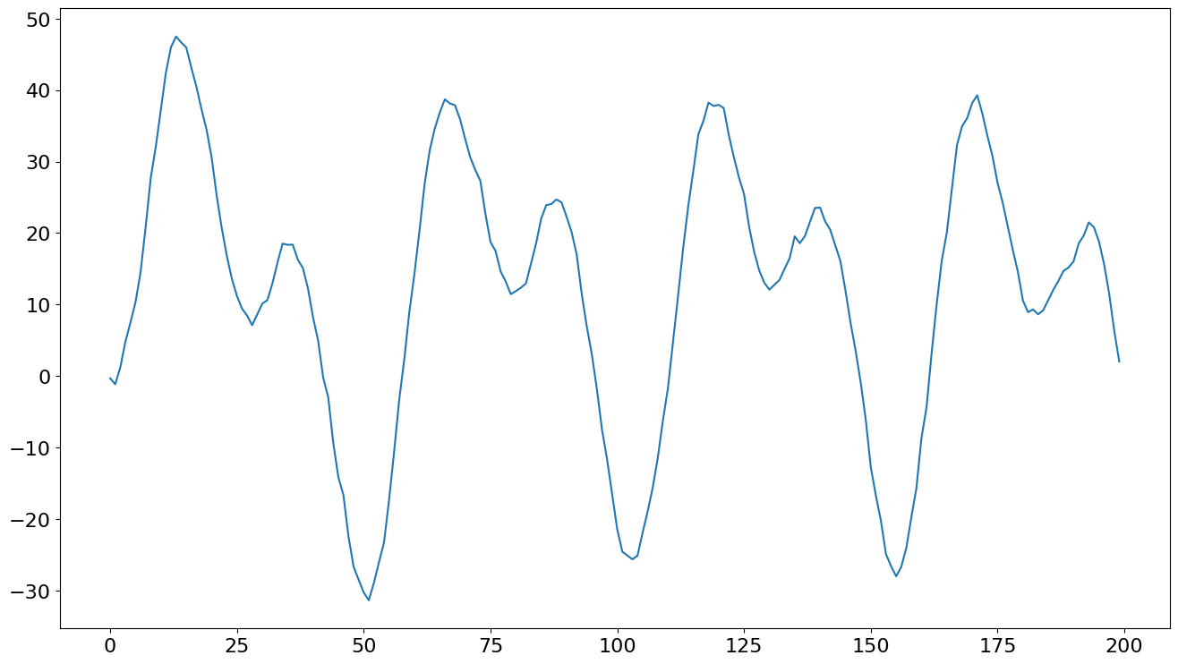
ここでは、フーリエ級数によって捉えられた週間の季節性を有するデータをシミュレートします。
[17]:
gen = np.random.default_rng(98765432101234567890)
idx = pd.RangeIndex(200)
det_proc = DeterministicProcess(idx, constant=True, period=52, fourier=2)
det_terms = det_proc.in_sample().to_numpy()
params = np.array([1.0, 3, -1, 4, -2])
exog = det_terms @ params
y = np.empty(200)
y[0] = det_terms[0] @ params + gen.standard_normal()
for i in range(1, 200):
    y[i] = 0.9 * y[i - 1] + det_terms[i] @ params + gen.standard_normal()
y = pd.Series(y, index=idx)
ax = y.plot()
次に、deterministicキーワード引数を使用してモデルを適合させます。seasonalはデフォルトでFalseですが、trendはデフォルトで"c"なので、変更する必要があります。
[18]:
from statsmodels.tsa.api import AutoReg

mod = AutoReg(y, 1, trend="n", deterministic=det_proc)
res = mod.fit()
print(res.summary())
                            AutoReg Model Results
==============================================================================
Dep. Variable:                      y   No. Observations:                  200
Model:                     AutoReg(1)   Log Likelihood                -270.964
Method:               Conditional MLE   S.D. of innovations              0.944
Date:                Thu, 03 Oct 2024   AIC                            555.927
Time:                        15:46:43   BIC                            578.980
Sample:                             1   HQIC                           565.258
                                  200
==============================================================================
                 coef    std err          z      P>|z|      [0.025      0.975]
------------------------------------------------------------------------------
const          0.8436      0.172      4.916      0.000       0.507       1.180
sin(1,52)      2.9738      0.160     18.587      0.000       2.660       3.287
cos(1,52)     -0.6771      0.284     -2.380      0.017      -1.235      -0.120
sin(2,52)      3.9951      0.099     40.336      0.000       3.801       4.189
cos(2,52)     -1.7206      0.264     -6.519      0.000      -2.238      -1.203
y.L1           0.9116      0.014     63.264      0.000       0.883       0.940
                                    Roots
=============================================================================
                  Real          Imaginary           Modulus         Frequency
-----------------------------------------------------------------------------
AR.1            1.0970           +0.0000j            1.0970            0.0000
-----------------------------------------------------------------------------
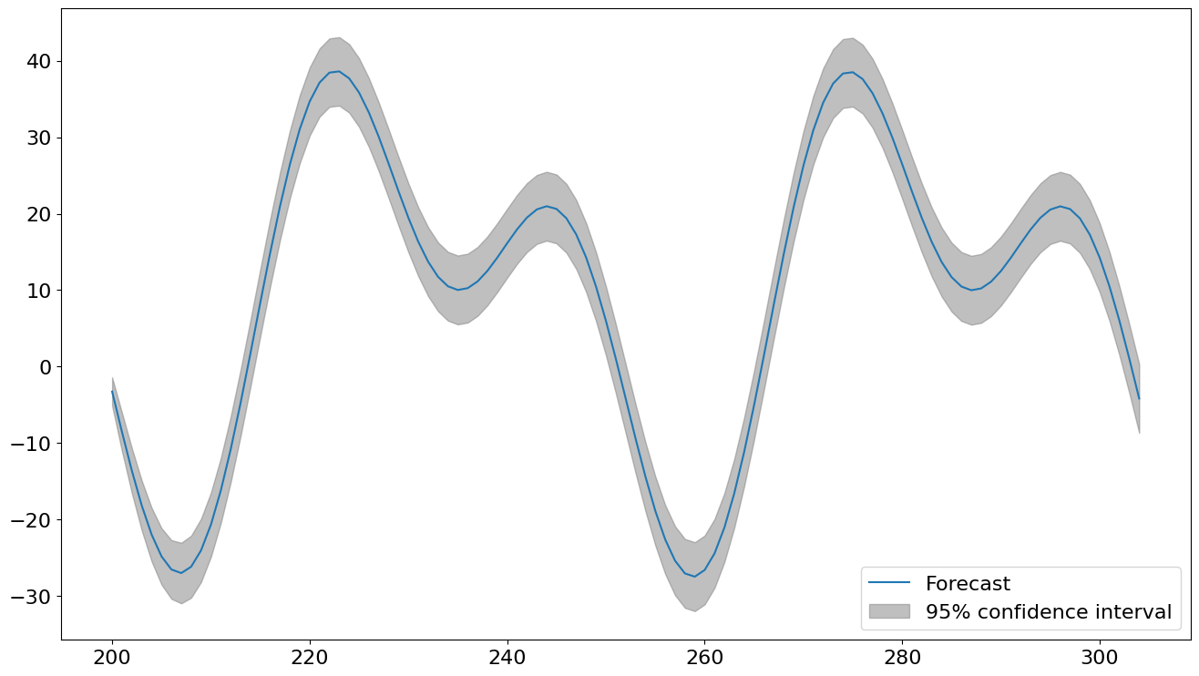
plot_predictを使用して、予測値とその予測区間を表示できます。サンプル外の決定論的値は、AutoRegに渡された決定論的プロセスによって自動的に生成されます。
[19]:
fig = res.plot_predict(200, 200 + 2 * 52, True)
[20]:
auto_reg_forecast = res.predict(200, 211)
auto_reg_forecast
[20]:
200    -3.253482
201    -8.555660
202   -13.607557
203   -18.152622
204   -21.950370
205   -24.790116
206   -26.503171
207   -26.972781
208   -26.141244
209   -24.013773
210   -20.658891
211   -16.205310
dtype: float64
他のモデルとの使用
他のモデルはDeterministicProcessを直接サポートしていません。代わりに、外生値をサポートするモデルに、決定論的項をexogとして手動で渡すことができます。
外生変数を持つSARIMAXは、SARIMA誤差を持つOLSであることに注意してください。モデルは次のようになります。
決定論的項のパラメータは、次の式に従って進化するAutoRegと直接比較できません。
\(x_t\)に決定論的項のみが含まれる場合、これらの2つの表現は同等です(\(\theta(L)=0\)、つまりMAがないと仮定)。
[21]:
from statsmodels.tsa.api import SARIMAX

det_proc = DeterministicProcess(idx, period=52, fourier=2)
det_terms = det_proc.in_sample()

mod = SARIMAX(y, order=(1, 0, 0), trend="c", exog=det_terms)
res = mod.fit(disp=False)
print(res.summary())
                               SARIMAX Results
==============================================================================
Dep. Variable:                      y   No. Observations:                  200
Model:               SARIMAX(1, 0, 0)   Log Likelihood                -293.381
Date:                Thu, 03 Oct 2024   AIC                            600.763
Time:                        15:46:44   BIC                            623.851
Sample:                             0   HQIC                           610.106
                                - 200
Covariance Type:                  opg
==============================================================================
                 coef    std err          z      P>|z|      [0.025      0.975]
------------------------------------------------------------------------------
intercept      0.0796      0.140      0.567      0.571      -0.196       0.355
sin(1,52)      9.1917      0.876     10.492      0.000       7.475      10.909
cos(1,52)    -17.4351      0.891    -19.576      0.000     -19.181     -15.689
sin(2,52)      1.2509      0.466      2.683      0.007       0.337       2.165
cos(2,52)    -17.1865      0.434    -39.582      0.000     -18.038     -16.335
ar.L1          0.9957      0.007    150.751      0.000       0.983       1.009
sigma2         1.0748      0.119      9.067      0.000       0.842       1.307
===================================================================================
Ljung-Box (L1) (Q):                   2.16   Jarque-Bera (JB):                 1.03
Prob(Q):                              0.14   Prob(JB):                         0.60
Heteroskedasticity (H):               0.71   Skew:                            -0.14
Prob(H) (two-sided):                  0.16   Kurtosis:                         2.78
===================================================================================

Warnings:
[1] Covariance matrix calculated using the outer product of gradients (complex-step).
予測は似ていますが、SARIMAXのパラメータはMLEを使用して推定されるのに対し、AutoRegはOLSを使用するため、異なります。
[22]:
sarimax_forecast = res.forecast(12, exog=det_proc.out_of_sample(12))
df = pd.concat([auto_reg_forecast, sarimax_forecast], axis=1)
df.columns = columns = ["AutoReg", "SARIMAX"]
df
[22]:
| AutoReg | SARIMAX | |
|---|---|---|
| 200 | -3.253482 | -2.956589 |
| 201 | -8.555660 | -7.985653 |
| 202 | -13.607557 | -12.794185 |
| 203 | -18.152622 | -17.131131 |
| 204 | -21.950370 | -20.760701 |
| 205 | -24.790116 | -23.475800 |
| 206 | -26.503171 | -25.109977 |
| 207 | -26.972781 | -25.547191 |
| 208 | -26.141244 | -24.728829 |
| 209 | -24.013773 | -22.657570 |
| 210 | -20.658891 | -19.397843 |
| 211 | -16.205310 | -15.072875 |