指数平滑法¶

ハインドマンとアタナソポウロスによる指数平滑法の優れた論文[1]の第7章を考えてみましょう。章で展開されるすべての例を実際に試していきます。

[1] Hyndman, Rob J., and George Athanasopoulos. Forecasting: principles and practice. OTexts, 2014.

データの読み込み¶

まず、いくつかのデータを読み込みます。便宜上、Rデータをノートブックに含めました。

[1]:

import os
import numpy as np
import pandas as pd
import matplotlib.pyplot as plt
from statsmodels.tsa.api import ExponentialSmoothing, SimpleExpSmoothing, Holt

%matplotlib inline

data = [
6565,
4733,
663,
6322,
2713,
5881,
3325,
1494,
0482,
792,
2689,
211,
]
index = pd.date_range(start="1996", end="2008", freq="Y")
oildata = pd.Series(data, index)

data = [
5534,
86,
8866,
9293,
8885,
8314,
0751,
9535,
1857,
5797,
5776,
4774,
0216,
3864,
5966,
]
index = pd.date_range(start="1990", end="2005", freq="Y")
air = pd.Series(data, index)

data = [
9177,
3072,
6626,
6394,
5158,
834,
309,
4742,
8307,
2867,
3311,
3724,
884,
2441,
6006,
2554,
4597,
4138,
7893,
3852,
2979,
3705,
5629,
1236,
7495,
2339,
9468,
6971,
4993,
2705,
2428,
]
index = pd.date_range(start="1970", end="2001", freq="Y")
livestock2 = pd.Series(data, index)

data = [407.9979, 403.4608, 413.8249, 428.105, 445.3387, 452.9942, 455.7402]
index = pd.date_range(start="2001", end="2008", freq="Y")
livestock3 = pd.Series(data, index)

data = [
7275,
0418,
3281,
3287,
2132,
3463,
4829,
9777,
9015,
1802,
7179,
4202,
2069,
8872,
9783,
7725,
5586,
8509,
0764,
6423,
7668,
1919,
3197,
9137,
]
index = pd.date_range(start="2005", end="2010-Q4", freq="QS-OCT")
aust = pd.Series(data, index)

/tmp/ipykernel_3946/536270367.py:23: FutureWarning: 'Y' is deprecated and will be removed in a future version, please use 'YE' instead.
  index = pd.date_range(start="1996", end="2008", freq="Y")
/tmp/ipykernel_3946/536270367.py:43: FutureWarning: 'Y' is deprecated and will be removed in a future version, please use 'YE' instead.
  index = pd.date_range(start="1990", end="2005", freq="Y")
/tmp/ipykernel_3946/536270367.py:79: FutureWarning: 'Y' is deprecated and will be removed in a future version, please use 'YE' instead.
  index = pd.date_range(start="1970", end="2001", freq="Y")
/tmp/ipykernel_3946/536270367.py:83: FutureWarning: 'Y' is deprecated and will be removed in a future version, please use 'YE' instead.
  index = pd.date_range(start="2001", end="2008", freq="Y")

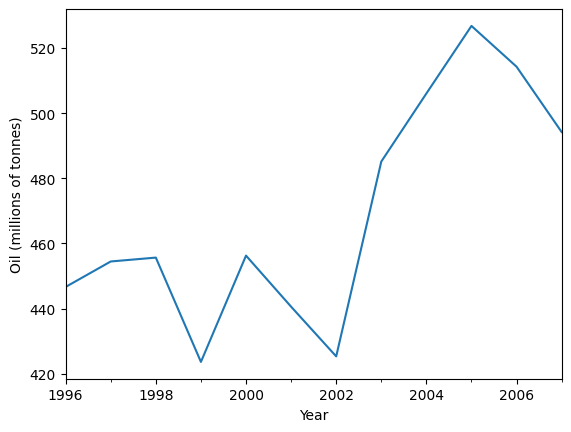
単純指数平滑法¶

単純指数平滑法を使用して、以下の石油データを予測してみましょう。

[2]:

ax = oildata.plot()
ax.set_xlabel("Year")
ax.set_ylabel("Oil (millions of tonnes)")
print("Figure 7.1: Oil production in Saudi Arabia from 1996 to 2007.")

Figure 7.1: Oil production in Saudi Arabia from 1996 to 2007.

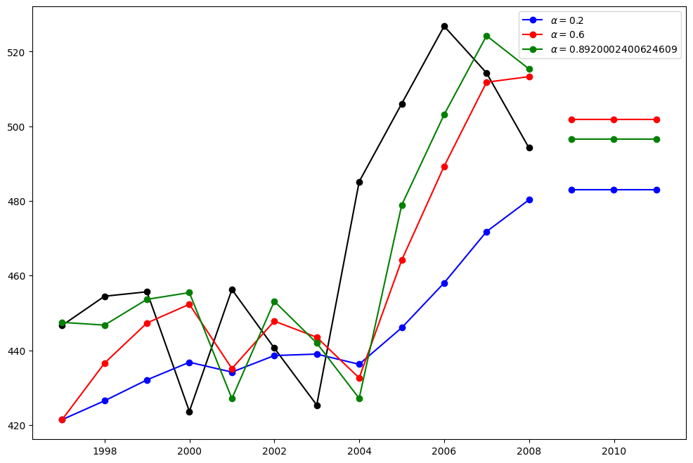
../../../_images/examples_notebooks_generated_exponential_smoothing_4_1.png

ここでは、単純指数平滑法の3つのバリアントを実行します。1. fit1では、自動最適化を使用せず、モデルに明示的に$\alpha=0.2$パラメーターを指定します。2. fit2では上記と同様に、$\alpha=0.6$を選択します。3. fit3では、statsmodelsが最適化された$\alpha$値を自動的に見つけられるようにします。これは推奨されるアプローチです。

[3]:

fit1 = SimpleExpSmoothing(oildata, initialization_method="heuristic").fit(
    smoothing_level=0.2, optimized=False
)
fcast1 = fit1.forecast(3).rename(r"$\alpha=0.2$")
fit2 = SimpleExpSmoothing(oildata, initialization_method="heuristic").fit(
    smoothing_level=0.6, optimized=False
)
fcast2 = fit2.forecast(3).rename(r"$\alpha=0.6$")
fit3 = SimpleExpSmoothing(oildata, initialization_method="estimated").fit()
fcast3 = fit3.forecast(3).rename(r"$\alpha=%s$" % fit3.model.params["smoothing_level"])

plt.figure(figsize=(12, 8))
plt.plot(oildata, marker="o", color="black")
plt.plot(fit1.fittedvalues, marker="o", color="blue")
(line1,) = plt.plot(fcast1, marker="o", color="blue")
plt.plot(fit2.fittedvalues, marker="o", color="red")
(line2,) = plt.plot(fcast2, marker="o", color="red")
plt.plot(fit3.fittedvalues, marker="o", color="green")
(line3,) = plt.plot(fcast3, marker="o", color="green")
plt.legend([line1, line2, line3], [fcast1.name, fcast2.name, fcast3.name])

[3]:

<matplotlib.legend.Legend at 0x7f4b3edd1930>

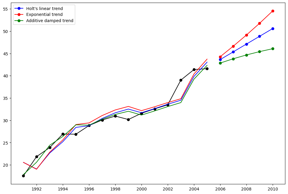
../../../_images/examples_notebooks_generated_exponential_smoothing_6_1.png

ホルト法¶

別の例を見てみましょう。今回は大気汚染データとホルト法を使用します。ここでも3つの例を当てはめます。1. fit1では、再度最適化ツールを使用せず、$\alpha=0.8$と$\beta=0.2$の明示的な値を指定します。2. fit2では、fit1と同じことを行いますが、ホルトの加法モデルではなく指数モデルを使用することを選択します。3. fit3では、ホルトの加法モデルの減衰バージョンを使用しますが、減衰パラメーター$\phi$を最適化し、$\alpha=0.8$と$\beta=0.2$の値を固定します。

[4]:

fit1 = Holt(air, initialization_method="estimated").fit(
    smoothing_level=0.8, smoothing_trend=0.2, optimized=False
)
fcast1 = fit1.forecast(5).rename("Holt's linear trend")
fit2 = Holt(air, exponential=True, initialization_method="estimated").fit(
    smoothing_level=0.8, smoothing_trend=0.2, optimized=False
)
fcast2 = fit2.forecast(5).rename("Exponential trend")
fit3 = Holt(air, damped_trend=True, initialization_method="estimated").fit(
    smoothing_level=0.8, smoothing_trend=0.2
)
fcast3 = fit3.forecast(5).rename("Additive damped trend")

plt.figure(figsize=(12, 8))
plt.plot(air, marker="o", color="black")
plt.plot(fit1.fittedvalues, color="blue")
(line1,) = plt.plot(fcast1, marker="o", color="blue")
plt.plot(fit2.fittedvalues, color="red")
(line2,) = plt.plot(fcast2, marker="o", color="red")
plt.plot(fit3.fittedvalues, color="green")
(line3,) = plt.plot(fcast3, marker="o", color="green")
plt.legend([line1, line2, line3], [fcast1.name, fcast2.name, fcast3.name])

[4]:

<matplotlib.legend.Legend at 0x7f4b3c76be20>

../../../_images/examples_notebooks_generated_exponential_smoothing_8_1.png

季節調整済みデータ¶

季節調整済みの家畜データを見てみましょう。5つのホルトモデルを当てはめます。以下の表を使用すると、指数モデルを使用した場合と加法モデルを使用した場合、および減衰モデルと非減衰モデルを使用した場合の結果を比較できます。

注：fit4では、$\phi=0.98$の固定値を提供することにより、パラメーター$\phi$を最適化することはできません。

[5]:

fit1 = SimpleExpSmoothing(livestock2, initialization_method="estimated").fit()
fit2 = Holt(livestock2, initialization_method="estimated").fit()
fit3 = Holt(livestock2, exponential=True, initialization_method="estimated").fit()
fit4 = Holt(livestock2, damped_trend=True, initialization_method="estimated").fit(
    damping_trend=0.98
)
fit5 = Holt(
    livestock2, exponential=True, damped_trend=True, initialization_method="estimated"
).fit()
params = [
    "smoothing_level",
    "smoothing_trend",
    "damping_trend",
    "initial_level",
    "initial_trend",
]
results = pd.DataFrame(
    index=[r"$\alpha$", r"$\beta$", r"$\phi$", r"$l_0$", "$b_0$", "SSE"],
    columns=["SES", "Holt's", "Exponential", "Additive", "Multiplicative"],
)
results["SES"] = [fit1.params[p] for p in params] + [fit1.sse]
results["Holt's"] = [fit2.params[p] for p in params] + [fit2.sse]
results["Exponential"] = [fit3.params[p] for p in params] + [fit3.sse]
results["Additive"] = [fit4.params[p] for p in params] + [fit4.sse]
results["Multiplicative"] = [fit5.params[p] for p in params] + [fit5.sse]
results

[5]:

	SES	ホルト法	指数	加法	乗法
$\alpha$	1.000000	0.974338	0.977642	0.978843	0.974912
$\beta$	NaN	0.000000	0.000000	0.000008	0.000000
$\phi$	NaN	NaN	NaN	0.980000	0.981646
$l_0$	263.917703	258.882683	260.335599	257.357716	258.951817
$b_0$	NaN	5.010856	1.013780	6.645297	1.038144
SSE	6761.350235	6004.138207	6104.194782	6036.597169	6081.995045

季節調整済みデータのプロット¶

次のプロットを使用すると、上記の表の当てはめのレベルと傾き/トレンドのコンポーネントを評価できます。

[6]:

for fit in [fit2, fit4]:
    pd.DataFrame(np.c_[fit.level, fit.trend]).rename(
        columns={0: "level", 1: "slope"}
    ).plot(subplots=True)
plt.show()
print(
    "Figure 7.4: Level and slope components for Holt’s linear trend method and the additive damped trend method."
)

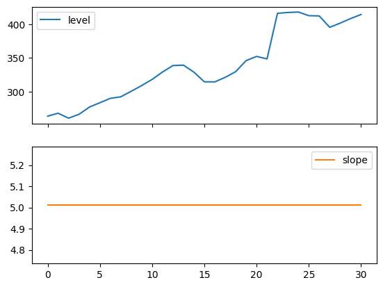
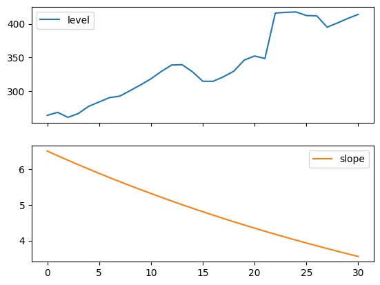
../../../_images/examples_notebooks_generated_exponential_smoothing_12_0.png

../../../_images/examples_notebooks_generated_exponential_smoothing_12_1.png

Figure 7.4: Level and slope components for Holt’s linear trend method and the additive damped trend method.

比較¶

ここでは、さまざまな加法、指数、および減衰の組み合わせについて、単純指数平滑法とホルト法を比較したプロットを作成します。すべてのモデルパラメーターは、statsmodelsによって最適化されます。

[7]:

fit1 = SimpleExpSmoothing(livestock2, initialization_method="estimated").fit()
fcast1 = fit1.forecast(9).rename("SES")
fit2 = Holt(livestock2, initialization_method="estimated").fit()
fcast2 = fit2.forecast(9).rename("Holt's")
fit3 = Holt(livestock2, exponential=True, initialization_method="estimated").fit()
fcast3 = fit3.forecast(9).rename("Exponential")
fit4 = Holt(livestock2, damped_trend=True, initialization_method="estimated").fit(
    damping_trend=0.98
)
fcast4 = fit4.forecast(9).rename("Additive Damped")
fit5 = Holt(
    livestock2, exponential=True, damped_trend=True, initialization_method="estimated"
).fit()
fcast5 = fit5.forecast(9).rename("Multiplicative Damped")

ax = livestock2.plot(color="black", marker="o", figsize=(12, 8))
livestock3.plot(ax=ax, color="black", marker="o", legend=False)
fcast1.plot(ax=ax, color="red", legend=True)
fcast2.plot(ax=ax, color="green", legend=True)
fcast3.plot(ax=ax, color="blue", legend=True)
fcast4.plot(ax=ax, color="cyan", legend=True)
fcast5.plot(ax=ax, color="magenta", legend=True)
ax.set_ylabel("Livestock, sheep in Asia (millions)")
plt.show()
print(
    "Figure 7.5: Forecasting livestock, sheep in Asia: comparing forecasting performance of non-seasonal methods."
)

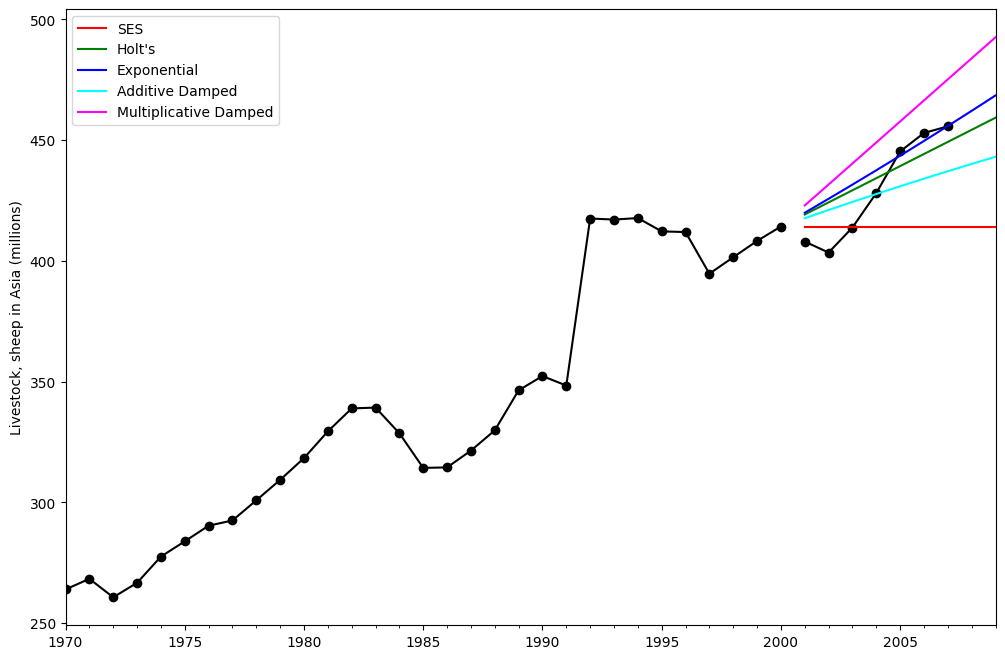
../../../_images/examples_notebooks_generated_exponential_smoothing_14_0.png

Figure 7.5: Forecasting livestock, sheep in Asia: comparing forecasting performance of non-seasonal methods.

ホルト＝ウィンタース法（季節性）¶

最後に、トレンドコンポーネントと季節コンポーネントを含む完全なホルト＝ウィンタースの季節指数平滑法を実行できます。statsmodelsでは、以下の例に示すように、すべての組み合わせが可能です。1. fit1 加法トレンド、期間がseason_length=4の加法季節性、およびボックス・コックス変換の使用。1. fit2 加法トレンド、期間がseason_length=4の乗法季節性、およびボックス・コックス変換の使用。1. fit3 減衰加法トレンド、期間がseason_length=4の加法季節性、およびボックス・コックス変換の使用。1. fit4 減衰加法トレンド、期間がseason_length=4の乗法季節性、およびボックス・コックス変換の使用。

プロットは、fit1とfit2の結果と予測を示しています。表を使用すると、結果とパラメーター化を比較できます。

[8]:

fit1 = ExponentialSmoothing(
    aust,
    seasonal_periods=4,
    trend="add",
    seasonal="add",
    use_boxcox=True,
    initialization_method="estimated",
).fit()
fit2 = ExponentialSmoothing(
    aust,
    seasonal_periods=4,
    trend="add",
    seasonal="mul",
    use_boxcox=True,
    initialization_method="estimated",
).fit()
fit3 = ExponentialSmoothing(
    aust,
    seasonal_periods=4,
    trend="add",
    seasonal="add",
    damped_trend=True,
    use_boxcox=True,
    initialization_method="estimated",
).fit()
fit4 = ExponentialSmoothing(
    aust,
    seasonal_periods=4,
    trend="add",
    seasonal="mul",
    damped_trend=True,
    use_boxcox=True,
    initialization_method="estimated",
).fit()
results = pd.DataFrame(
    index=[r"$\alpha$", r"$\beta$", r"$\phi$", r"$\gamma$", r"$l_0$", "$b_0$", "SSE"]
)
params = [
    "smoothing_level",
    "smoothing_trend",
    "damping_trend",
    "smoothing_seasonal",
    "initial_level",
    "initial_trend",
]
results["Additive"] = [fit1.params[p] for p in params] + [fit1.sse]
results["Multiplicative"] = [fit2.params[p] for p in params] + [fit2.sse]
results["Additive Dam"] = [fit3.params[p] for p in params] + [fit3.sse]
results["Multiplica Dam"] = [fit4.params[p] for p in params] + [fit4.sse]

ax = aust.plot(
    figsize=(10, 6),
    marker="o",
    color="black",
    title="Forecasts from Holt-Winters' multiplicative method",
)
ax.set_ylabel("International visitor night in Australia (millions)")
ax.set_xlabel("Year")
fit1.fittedvalues.plot(ax=ax, style="--", color="red")
fit2.fittedvalues.plot(ax=ax, style="--", color="green")

fit1.forecast(8).rename("Holt-Winters (add-add-seasonal)").plot(
    ax=ax, style="--", marker="o", color="red", legend=True
)
fit2.forecast(8).rename("Holt-Winters (add-mul-seasonal)").plot(
    ax=ax, style="--", marker="o", color="green", legend=True
)

plt.show()
print(
    "Figure 7.6: Forecasting international visitor nights in Australia using Holt-Winters method with both additive and multiplicative seasonality."
)

results

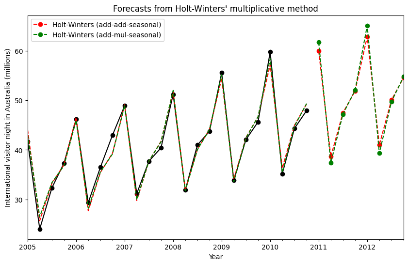
../../../_images/examples_notebooks_generated_exponential_smoothing_16_0.png

Figure 7.6: Forecasting international visitor nights in Australia using Holt-Winters method with both additive and multiplicative seasonality.

[8]:

	加法	乗法	加法ダム	乗法ダム
$\alpha$	1.490116e-08	1.490116e-08	1.490116e-08	1.490116e-08
$\beta$	1.409865e-08	0.000000e+00	6.490845e-09	5.042120e-09
$\phi$	NaN	NaN	9.430416e-01	9.536043e-01
$\gamma$	7.066690e-16	1.514304e-16	1.169213e-15	0.000000e+00
$l_0$	1.119348e+01	1.106382e+01	1.084022e+01	9.899305e+00
$b_0$	1.205396e-01	1.198963e-01	2.456750e-01	1.975449e-01
SSE	4.402746e+01	3.611262e+01	3.527620e+01	3.062033e+01

内部構造¶

指数平滑モデルの内部構造にアクセスできます。

ここでは、元の値$y_t$、レベル$l_t$、トレンド$b_t$、季節性$s_t$、および適合値$\hat{y}_t$を並べて表示できるいくつかの表を示します。これらの値は、ボックス・コックス変換なしで適合が実行された場合にのみ、元のデータの空間で意味のある値を持つことに注意してください。

[9]:

fit1 = ExponentialSmoothing(
    aust,
    seasonal_periods=4,
    trend="add",
    seasonal="add",
    initialization_method="estimated",
).fit()
fit2 = ExponentialSmoothing(
    aust,
    seasonal_periods=4,
    trend="add",
    seasonal="mul",
    initialization_method="estimated",
).fit()

[10]:

df = pd.DataFrame(
    np.c_[aust, fit1.level, fit1.trend, fit1.season, fit1.fittedvalues],
    columns=[r"$y_t$", r"$l_t$", r"$b_t$", r"$s_t$", r"$\hat{y}_t$"],
    index=aust.index,
)
forecasts = fit1.forecast(8).rename(r"$\hat{y}_t$").to_frame()
df = pd.concat([df, forecasts], axis=0, sort=True)

[11]:

df = pd.DataFrame(
    np.c_[aust, fit2.level, fit2.trend, fit2.season, fit2.fittedvalues],
    columns=[r"$y_t$", r"$l_t$", r"$b_t$", r"$s_t$", r"$\hat{y}_t$"],
    index=aust.index,
)
forecasts = fit2.forecast(8).rename(r"$\hat{y}_t$").to_frame()
df = pd.concat([df, forecasts], axis=0, sort=True)

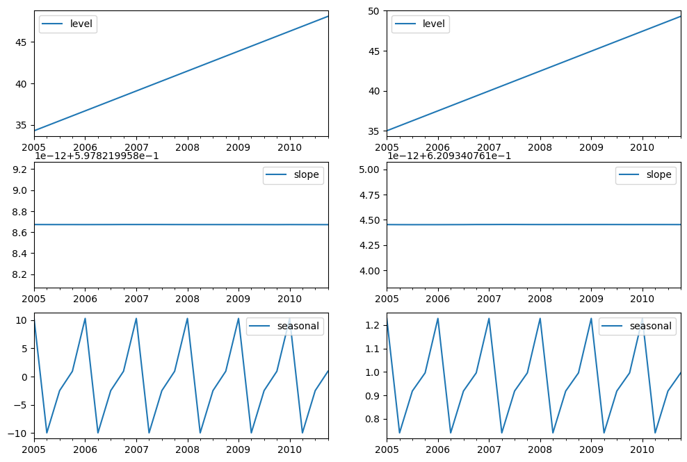
最後に、モデルのレベル、傾き/トレンド、および季節コンポーネントを見てみましょう。

[12]:

states1 = pd.DataFrame(
    np.c_[fit1.level, fit1.trend, fit1.season],
    columns=["level", "slope", "seasonal"],
    index=aust.index,
)
states2 = pd.DataFrame(
    np.c_[fit2.level, fit2.trend, fit2.season],
    columns=["level", "slope", "seasonal"],
    index=aust.index,
)
fig, [[ax1, ax4], [ax2, ax5], [ax3, ax6]] = plt.subplots(3, 2, figsize=(12, 8))
states1[["level"]].plot(ax=ax1)
states1[["slope"]].plot(ax=ax2)
states1[["seasonal"]].plot(ax=ax3)
states2[["level"]].plot(ax=ax4)
states2[["slope"]].plot(ax=ax5)
states2[["seasonal"]].plot(ax=ax6)
plt.show()

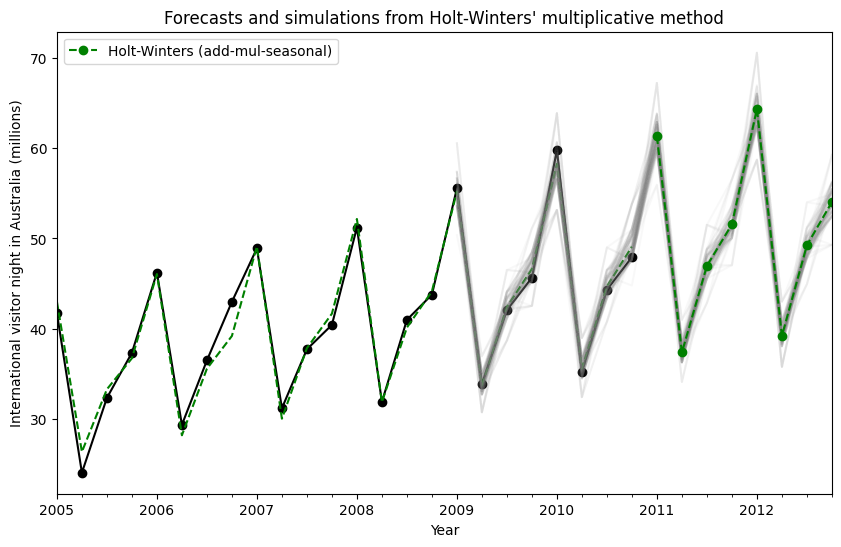
../../../_images/examples_notebooks_generated_exponential_smoothing_22_0.png

シミュレーションと信頼区間¶

状態空間の定式化を使用することにより、将来の値のシミュレーションを実行できます。数学的な詳細は、ハインドマンとアタナソポウロス[2]、およびHoltWintersResults.simulateのドキュメントで説明されています。

[2]の例と同様に、加法トレンド、乗法季節性、および乗法誤差を持つモデルを使用します。将来の8ステップまでシミュレーションし、1000回のシミュレーションを実行します。下の図でわかるように、シミュレーションは予測値と非常によく一致しています。

[2] Hyndman, Rob J., and George Athanasopoulos. Forecasting: principles and practice, 2nd edition. OTexts, 2018.

[13]:

fit = ExponentialSmoothing(
    aust,
    seasonal_periods=4,
    trend="add",
    seasonal="mul",
    initialization_method="estimated",
).fit()
simulations = fit.simulate(8, repetitions=100, error="mul")

ax = aust.plot(
    figsize=(10, 6),
    marker="o",
    color="black",
    title="Forecasts and simulations from Holt-Winters' multiplicative method",
)
ax.set_ylabel("International visitor night in Australia (millions)")
ax.set_xlabel("Year")
fit.fittedvalues.plot(ax=ax, style="--", color="green")
simulations.plot(ax=ax, style="-", alpha=0.05, color="grey", legend=False)
fit.forecast(8).rename("Holt-Winters (add-mul-seasonal)").plot(
    ax=ax, style="--", marker="o", color="green", legend=True
)
plt.show()

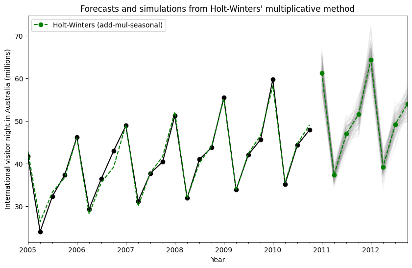
../../../_images/examples_notebooks_generated_exponential_smoothing_24_0.png

シミュレーションは、時間の異なる時点で開始することもでき、ランダムノイズを選択するための複数のオプションがあります。

[14]:

fit = ExponentialSmoothing(
    aust,
    seasonal_periods=4,
    trend="add",
    seasonal="mul",
    initialization_method="estimated",
).fit()
simulations = fit.simulate(
    16, anchor="2009-01-01", repetitions=100, error="mul", random_errors="bootstrap"
)

ax = aust.plot(
    figsize=(10, 6),
    marker="o",
    color="black",
    title="Forecasts and simulations from Holt-Winters' multiplicative method",
)
ax.set_ylabel("International visitor night in Australia (millions)")
ax.set_xlabel("Year")
fit.fittedvalues.plot(ax=ax, style="--", color="green")
simulations.plot(ax=ax, style="-", alpha=0.05, color="grey", legend=False)
fit.forecast(8).rename("Holt-Winters (add-mul-seasonal)").plot(
    ax=ax, style="--", marker="o", color="green", legend=True
)
plt.show()

../../../_images/examples_notebooks_generated_exponential_smoothing_26_0.png

最終更新日：2024年10月03日