LOESSを用いた季節・トレンド分解 (STL)¶

このノートブックは、STLを使用して時系列をトレンド、季節、残差の3つの成分に分解する方法を示しています。STLはLOESS（局所的に重み付けされた散布図平滑化）を使用して、3つの成分の滑らかな推定値を抽出します。STLの主要な入力は次のとおりです。

season - 季節スムージングの長さ。奇数でなければなりません。
trend - トレンドスムージングの長さ。通常はseasonの約150％。奇数でseasonより大きくする必要があります。
low_pass - ローパス推定ウィンドウの長さ。通常は、データの周期性よりも大きい最小の奇数。

まず、必要なパッケージをインポートし、グラフィックス環境を準備し、データを準備します。

[1]:

import matplotlib.pyplot as plt
import pandas as pd
import seaborn as sns
from pandas.plotting import register_matplotlib_converters

register_matplotlib_converters()
sns.set_style("darkgrid")

[2]:

plt.rc("figure", figsize=(16, 12))
plt.rc("font", size=13)

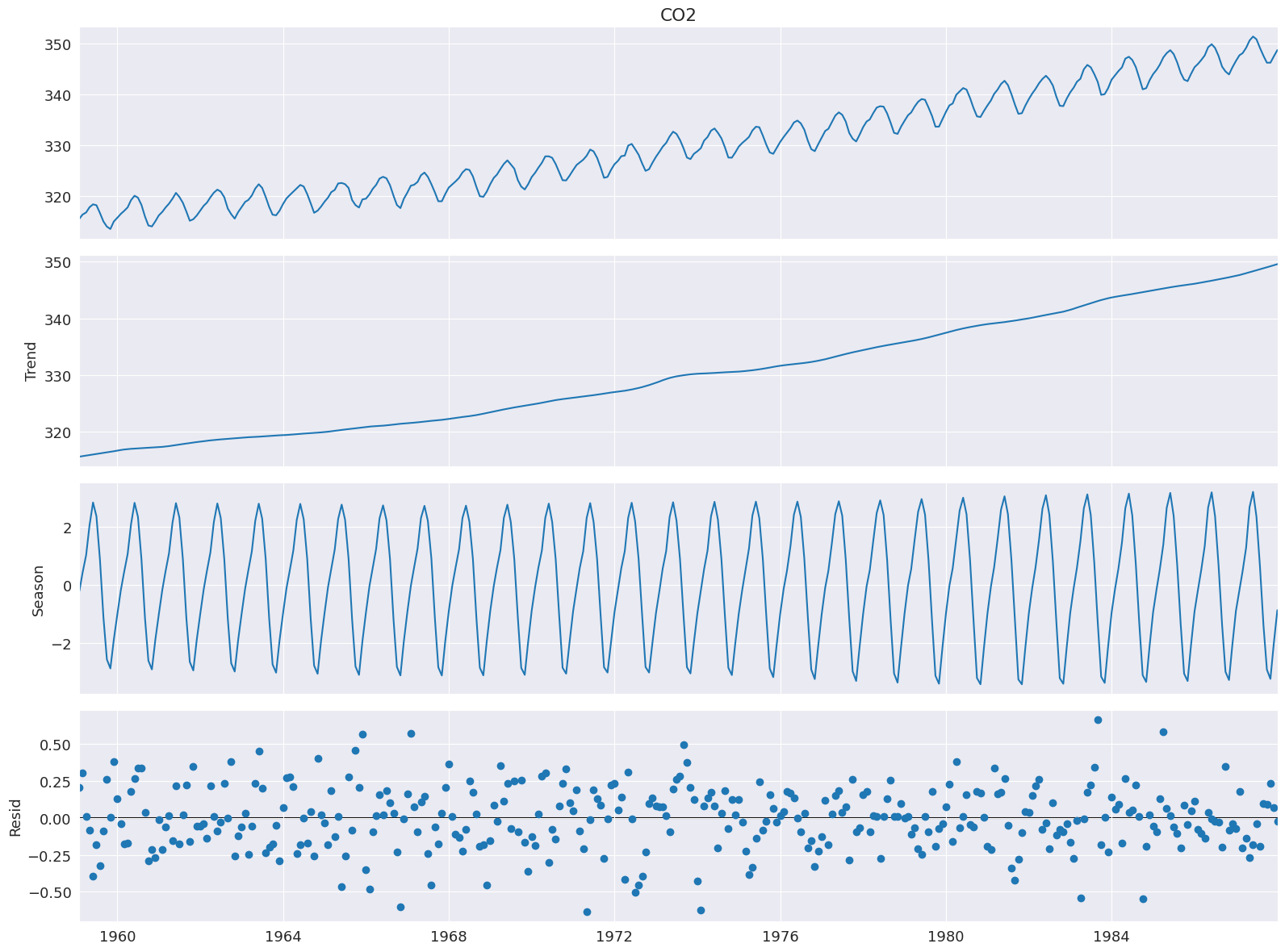
大気中のCO2¶

Cleveland, Cleveland, McRae, and Terpenning (1990)の例ではCO2データを使用しており、以下にリストされています。この月次データ（1959年1月から1987年12月）は、サンプル全体で明確なトレンドと季節性がみられます。

[3]:

co2 = [
58,
39,
79,
82,
39,
22,
68,
01,
02,
55,
02,
75,
52,
10,
79,
22,
08,
70,
27,
99,
24,
05,
05,
23,
92,
76,
54,
49,
64,
85,
70,
96,
17,
47,
19,
17,
12,
72,
79,
68,
28,
89,
79,
56,
46,
59,
85,
87,
87,
25,
13,
49,
34,
62,
85,
87,
36,
24,
13,
46,
57,
23,
89,
54,
20,
90,
42,
60,
73,
15,
94,
91,
73,
78,
23,
49,
59,
35,
61,
24,
23,
76,
36,
50,
35,
40,
22,
45,
80,
50,
16,
09,
26,
66,
47,
70,
06,
23,
78,
10,
63,
79,
34,
73,
00,
99,
41,
68,
30,
89,
59,
65,
30,
15,
88,
80,
99,
86,
88,
36,
59,
23,
34,
33,
03,
24,
39,
16,
87,
31,
34,
74,
61,
58,
55,
81,
82,
53,
29,
66,
12,
09,
01,
10,
12,
62,
16,
94,
15,
79,
53,
65,
60,
78,
13,
26,
93,
84,
96,
93,
25,
24,
13,
42,
97,
29,
56,
73,
73,
70,
46,
70,
66,
22,
02,
39,
58,
27,
30,
81,
44,
89,
62,
85,
29,
44,
35,
58,
58,
55,
56,
73,
45,
98,
63,
88,
63,
53,
90,
08,
59,
31,
44,
64,
62,
45,
36,
46,
84,
29,
04,
88,
23,
83,
18,
50,
80,
22,
54,
82,
45,
97,
65,
40,
28,
73,
05,
54,
65,
06,
32,
39,
66,
56,
24,
39,
43,
22,
61,
78,
88,
43,
61,
53,
06,
92,
39,
72,
64,
65,
07,
53,
82,
19,
89,
56,
22,
92,
26,
27,
66,
54,
71,
79,
79,
06,
93,
02,
65,
80,
01,
94,
17,
28,
76,
05,
18,
04,
16,
01,
64,
91,
72,
52,
75,
68,
14,
37,
32,
45,
05,
91,
77,
30,
98,
41,
89,
03,
19,
87,
74,
55,
28,
00,
37,
74,
36,
19,
97,
20,
76,
96,
82,
82,
24,
09,
66,
90,
27,
21,
88,
58,
99,
31,
98,
72,
63,
24,
83,
10,
52,
43,
48,
89,
29,
54,
66,
07,
12,
55,
34,
80,
10,
54,
20,
20,
44,
67,
]
co2 = pd.Series(
    co2, index=pd.date_range("1-1-1959", periods=len(co2), freq="M"), name="CO2"
)
co2.describe()

/tmp/ipykernel_3881/1071343913.py:352: FutureWarning: 'M' is deprecated and will be removed in a future version, please use 'ME' instead.
  co2, index=pd.date_range("1-1-1959", periods=len(co2), freq="M"), name="CO2"

[3]:

count    348.000000
mean     330.123879
std       10.059747
min      313.550000
25%      321.302500
50%      328.820000
75%      338.002500
max      351.340000
Name: CO2, dtype: float64

分解には、データ系列という1つの入力が必要です。データ系列に頻度がない場合は、periodも指定する必要があります。seasonalのデフォルト値は7なので、ほとんどのアプリケーションでは変更する必要があります。

[4]:

from statsmodels.tsa.seasonal import STL

stl = STL(co2, seasonal=13)
res = stl.fit()
fig = res.plot()

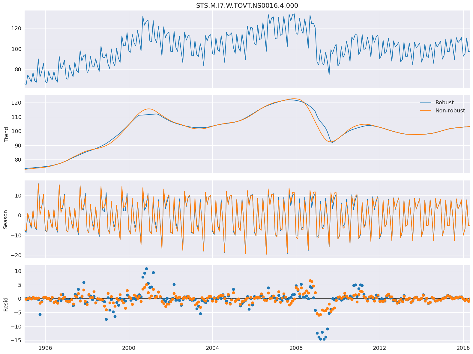
../../../_images/examples_notebooks_generated_stl_decomposition_6_0.png

頑健なフィッティング¶

robustを設定すると、LOESSの推定時にデータを再重み付けするデータ依存の重み付け関数を使用します（LOWESSを使用しています）。頑健な推定を使用すると、下側のプロットに表示されているような大きな誤差をモデルが許容できます。

ここでは、EUにおける電気機器生産量を測定する系列を使用します。

[5]:

from statsmodels.datasets import elec_equip as ds

elec_equip = ds.load().data.iloc[:, 0]

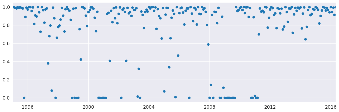
次に、頑健な重み付けありとなしでモデルを推定します。違いはわずかで、2008年の金融危機中に最も顕著です。頑健でない推定では、すべての観測値に等しい重み付けがされ、平均してより小さな誤差が生じます。重みは0から1の間で変化します。

[6]:

def add_stl_plot(fig, res, legend):
    """Add 3 plots from a second STL fit"""
    axs = fig.get_axes()
    comps = ["trend", "seasonal", "resid"]
    for ax, comp in zip(axs[1:], comps):
        series = getattr(res, comp)
        if comp == "resid":
            ax.plot(series, marker="o", linestyle="none")
        else:
            ax.plot(series)
            if comp == "trend":
                ax.legend(legend, frameon=False)

stl = STL(elec_equip, period=12, robust=True)
res_robust = stl.fit()
fig = res_robust.plot()
res_non_robust = STL(elec_equip, period=12, robust=False).fit()
add_stl_plot(fig, res_non_robust, ["Robust", "Non-robust"])

../../../_images/examples_notebooks_generated_stl_decomposition_10_0.png

[7]:

fig = plt.figure(figsize=(16, 5))
lines = plt.plot(res_robust.weights, marker="o", linestyle="none")
ax = plt.gca()
xlim = ax.set_xlim(elec_equip.index[0], elec_equip.index[-1])

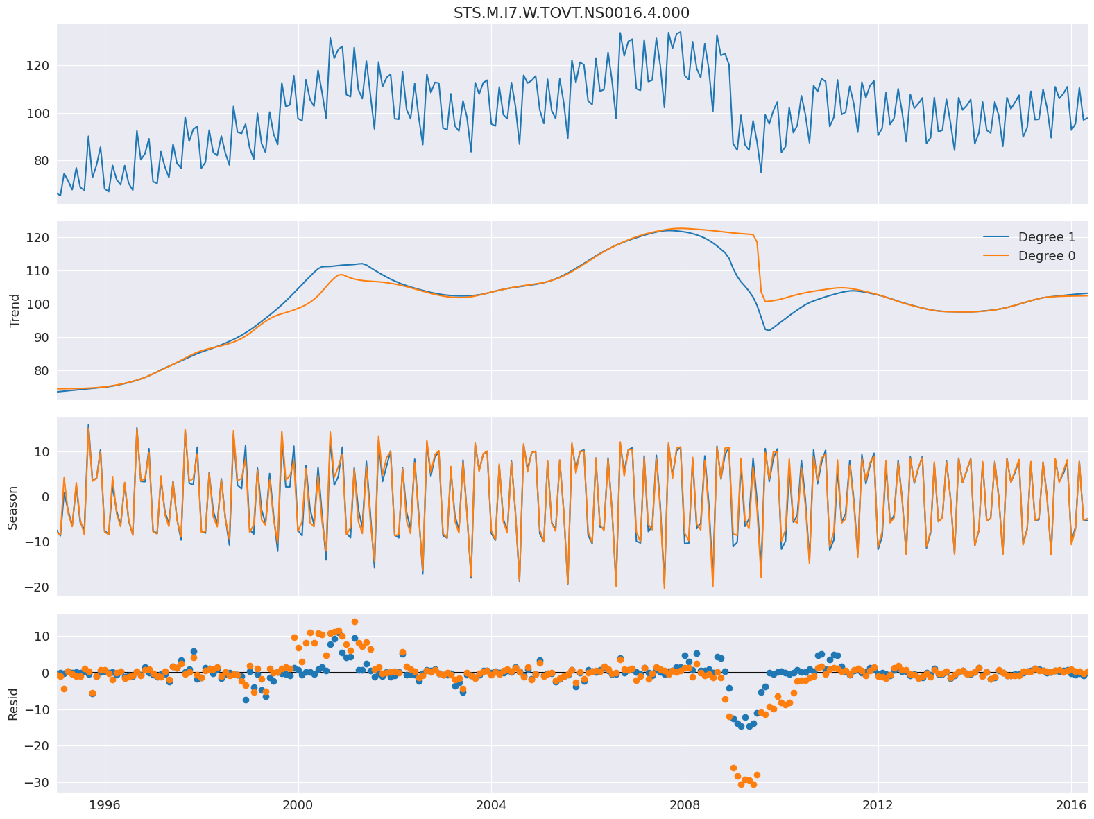
../../../_images/examples_notebooks_generated_stl_decomposition_11_0.png

LOESSの次数¶

デフォルトの設定では、定数とトレンドの両方を使用してLOESSモデルを推定します。COMPONENT_degを0に設定することで、定数のみを含めるように変更できます。ここでは、2008年の金融危機周辺のトレンドを除けば、次数はほとんど影響しません。

[8]:

stl = STL(
    elec_equip, period=12, seasonal_deg=0, trend_deg=0, low_pass_deg=0, robust=True
)
res_deg_0 = stl.fit()
fig = res_robust.plot()
add_stl_plot(fig, res_deg_0, ["Degree 1", "Degree 0"])

../../../_images/examples_notebooks_generated_stl_decomposition_13_0.png

パフォーマンス¶

STL分解の計算コストを削減するために、3つのオプションを使用できます。

seasonal_jump
trend_jump
low_pass_jump

これらの値が0以外の場合、コンポーネントCOMPONENTのLOESSはCOMPONENT_jump個の観測値ごとにのみ推定され、線形補間が点間で使用されます。これらの値は、通常、seasonal、trend、low_passのサイズのおよそ10～20％を超えるべきではありません。

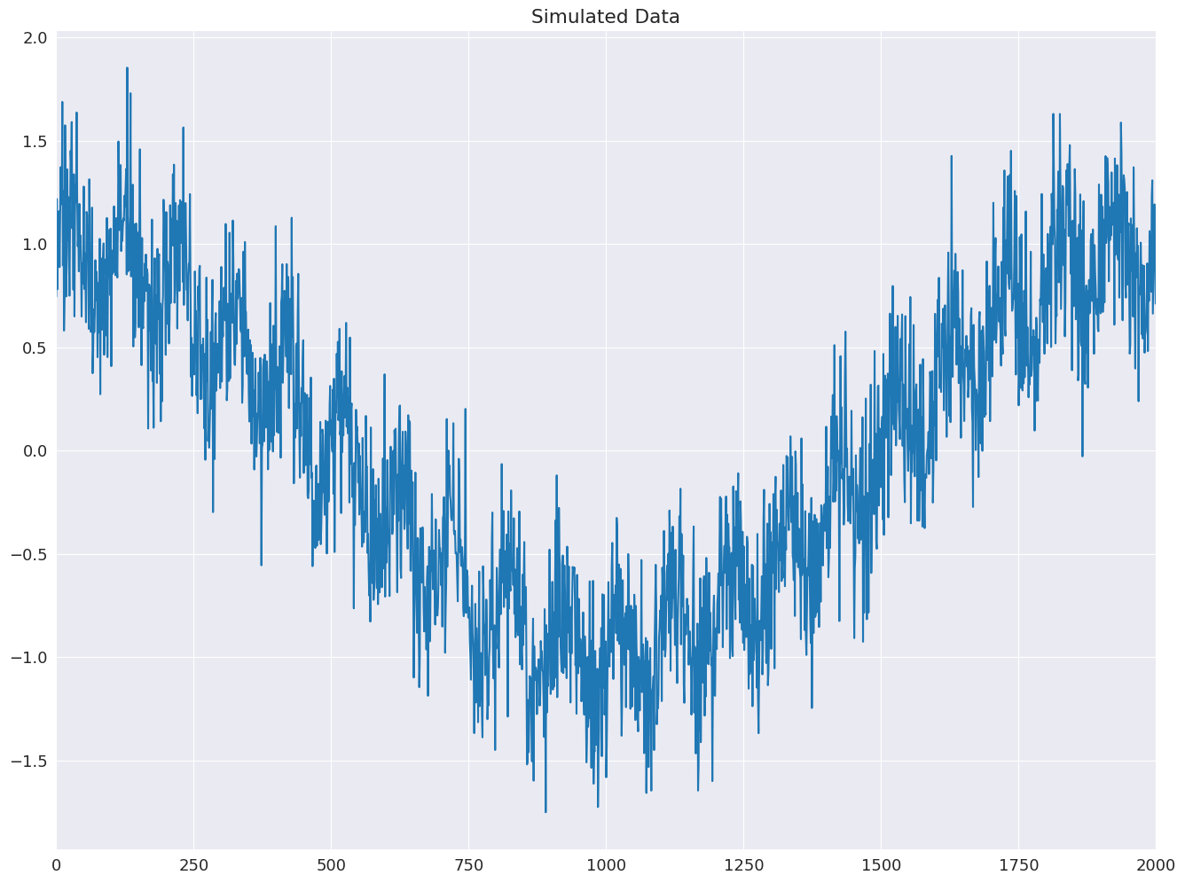
以下の例は、低周波の余弦トレンドと正弦波の季節パターンを持つシミュレートされたデータを使用して、これらが計算コストを15分の1に削減する方法を示しています。

[9]:

import numpy as np

rs = np.random.RandomState(0xA4FD94BC)
tau = 2000
t = np.arange(tau)
period = int(0.05 * tau)
seasonal = period + ((period % 2) == 0)  # Ensure odd
e = 0.25 * rs.standard_normal(tau)
y = np.cos(t / tau * 2 * np.pi) + 0.25 * np.sin(t / period * 2 * np.pi) + e
plt.plot(y)
plt.title("Simulated Data")
xlim = plt.gca().set_xlim(0, tau)

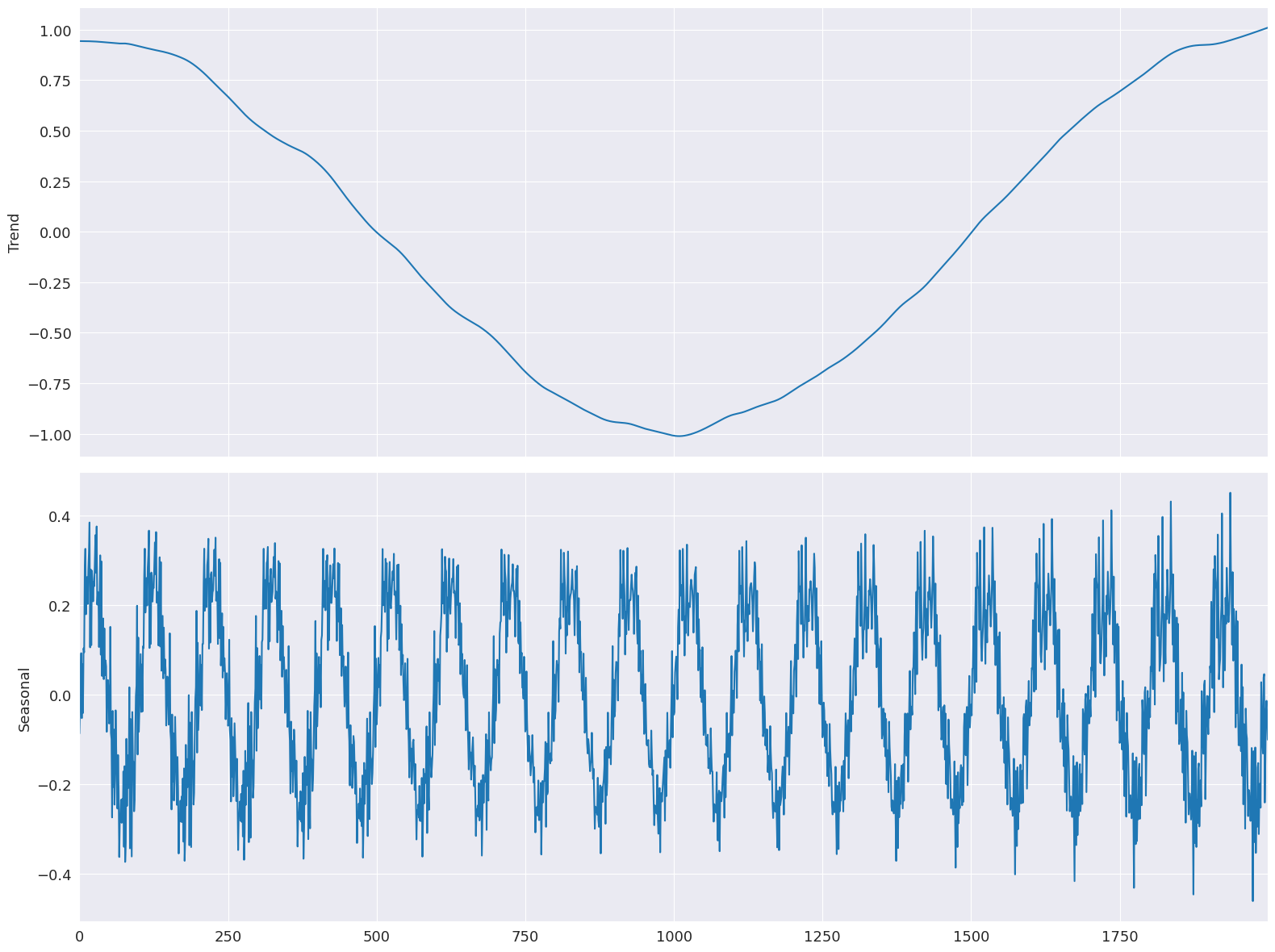
../../../_images/examples_notebooks_generated_stl_decomposition_15_0.png

まず、すべてのジャンプが1に等しいベースラインモデルを推定します。

[10]:

mod = STL(y, period=period, seasonal=seasonal)
%timeit mod.fit()
res = mod.fit()
fig = res.plot(observed=False, resid=False)

284 ms ± 38.9 ms per loop (mean ± std. dev. of 7 runs, 1 loop each)

../../../_images/examples_notebooks_generated_stl_decomposition_17_1.png

ジャンプはすべてウィンドウ長の15％に設定されます。制限された線形補間は、モデルの適合性にほとんど影響を与えません。

[11]:

low_pass_jump = seasonal_jump = int(0.15 * (period + 1))
trend_jump = int(0.15 * 1.5 * (period + 1))
mod = STL(
    y,
    period=period,
    seasonal=seasonal,
    seasonal_jump=seasonal_jump,
    trend_jump=trend_jump,
    low_pass_jump=low_pass_jump,
)
%timeit mod.fit()
res = mod.fit()
fig = res.plot(observed=False, resid=False)

22.9 ms ± 1.04 ms per loop (mean ± std. dev. of 7 runs, 10 loops each)

../../../_images/examples_notebooks_generated_stl_decomposition_19_1.png

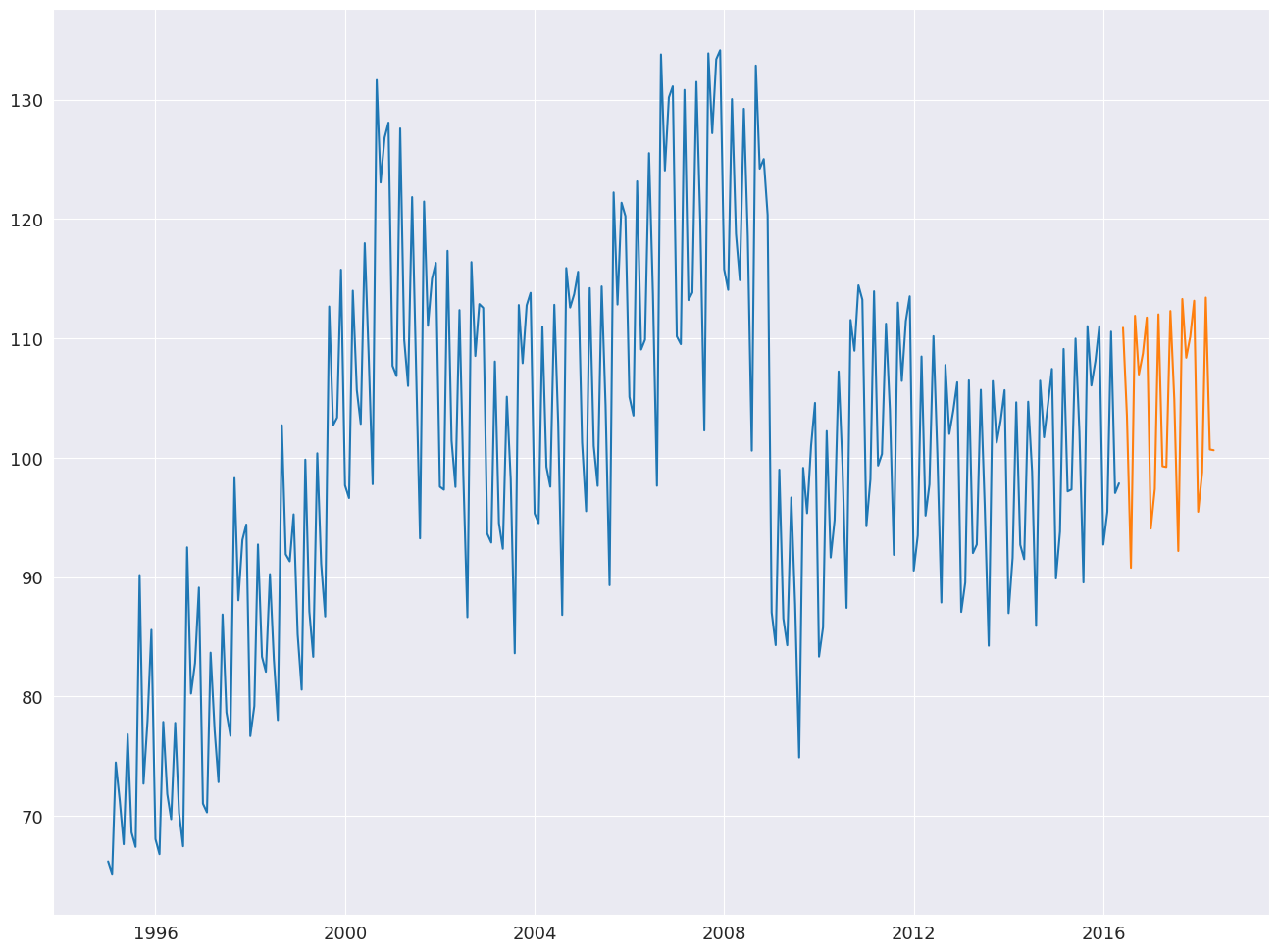
STLを用いた予測¶

STLForecastは、STLを使用して季節性を除去し、標準的な時系列モデルを使用してトレンドと循環成分を予測するプロセスを簡素化します。

ここでは、STLを使用して季節性を処理し、次にARIMA(1,1,0)を使用して季節調整済みのデータをモデル化します。季節成分は、以下の完全なサイクルを見つけることから予測されます。

\[E[S_{T+h}|\mathcal{F}_T]=\hat{S}_{T-k}\]

ここで、\(k= m - h + m \lfloor \frac{h-1}{m} \rfloor\)です。予測では、ARIMA予測に季節成分予測が自動的に追加されます。

[12]:

from statsmodels.tsa.arima.model import ARIMA
from statsmodels.tsa.forecasting.stl import STLForecast

elec_equip.index.freq = elec_equip.index.inferred_freq
stlf = STLForecast(elec_equip, ARIMA, model_kwargs=dict(order=(1, 1, 0), trend="t"))
stlf_res = stlf.fit()

forecast = stlf_res.forecast(24)
plt.plot(elec_equip)
plt.plot(forecast)
plt.show()

../../../_images/examples_notebooks_generated_stl_decomposition_21_0.png

summaryには、時系列モデルとSTL分解の両方の情報が含まれています。

[13]:

print(stlf_res.summary())

                    STL Decomposition and SARIMAX Results
==============================================================================
Dep. Variable:                      y   No. Observations:                  257
Model:                 ARIMA(1, 1, 0)   Log Likelihood                -522.434
Date:                Thu, 03 Oct 2024   AIC                           1050.868
Time:                        15:45:57   BIC                           1061.504
Sample:                    01-01-1995   HQIC                          1055.146
                         - 05-01-2016
Covariance Type:                  opg
==============================================================================
                 coef    std err          z      P>|z|      [0.025      0.975]
------------------------------------------------------------------------------
x1             0.1171      0.118      0.995      0.320      -0.113       0.348
ar.L1         -0.0435      0.049     -0.880      0.379      -0.140       0.053
sigma2         3.4682      0.188     18.406      0.000       3.099       3.837
===================================================================================
Ljung-Box (L1) (Q):                   0.01   Jarque-Bera (JB):               223.01
Prob(Q):                              0.92   Prob(JB):                         0.00
Heteroskedasticity (H):               0.33   Skew:                            -0.26
Prob(H) (two-sided):                  0.00   Kurtosis:                         7.54
                                STL Configuration
=================================================================================
Period:                            12       Trend Length:                      23
Seasonal:                           7       Trend deg:                          1
Seasonal deg:                       1       Trend jump:                         1
Seasonal jump:                      1       Low pass:                          13
Robust:                         False       Low pass deg:                       1
---------------------------------------------------------------------------------

Warnings:
[1] Covariance matrix calculated using the outer product of gradients (complex-step).

最終更新日：2024年10月3日