時系列フィルター
[1]:
%matplotlib inline
[2]:
import pandas as pd
import matplotlib.pyplot as plt

import statsmodels.api as sm
[3]:
dta = sm.datasets.macrodata.load_pandas().data
[4]:
index = pd.Index(sm.tsa.datetools.dates_from_range("1959Q1", "2009Q3"))
print(index)
DatetimeIndex(['1959-03-31', '1959-06-30', '1959-09-30', '1959-12-31',
               '1960-03-31', '1960-06-30', '1960-09-30', '1960-12-31',
               '1961-03-31', '1961-06-30',
               ...
               '2007-06-30', '2007-09-30', '2007-12-31', '2008-03-31',
               '2008-06-30', '2008-09-30', '2008-12-31', '2009-03-31',
               '2009-06-30', '2009-09-30'],
              dtype='datetime64[ns]', length=203, freq=None)
[5]:
dta.index = index
del dta["year"]
del dta["quarter"]
[6]:
print(sm.datasets.macrodata.NOTE)
::
    Number of Observations - 203

    Number of Variables - 14

    Variable name definitions::

        year      - 1959q1 - 2009q3
        quarter   - 1-4
        realgdp   - Real gross domestic product (Bil. of chained 2005 US$,
                    seasonally adjusted annual rate)
        realcons  - Real personal consumption expenditures (Bil. of chained
                    2005 US$, seasonally adjusted annual rate)
        realinv   - Real gross private domestic investment (Bil. of chained
                    2005 US$, seasonally adjusted annual rate)
        realgovt  - Real federal consumption expenditures & gross investment
                    (Bil. of chained 2005 US$, seasonally adjusted annual rate)
        realdpi   - Real private disposable income (Bil. of chained 2005
                    US$, seasonally adjusted annual rate)
        cpi       - End of the quarter consumer price index for all urban
                    consumers: all items (1982-84 = 100, seasonally adjusted).
        m1        - End of the quarter M1 nominal money stock (Seasonally
                    adjusted)
        tbilrate  - Quarterly monthly average of the monthly 3-month
                    treasury bill: secondary market rate
        unemp     - Seasonally adjusted unemployment rate (%)
        pop       - End of the quarter total population: all ages incl. armed
                    forces over seas
        infl      - Inflation rate (ln(cpi_{t}/cpi_{t-1}) * 400)
        realint   - Real interest rate (tbilrate - infl)
[7]:
print(dta.head(10))
             realgdp  realcons  realinv  realgovt  realdpi    cpi     m1  \
1959-03-31  2710.349    1707.4  286.898   470.045   1886.9  28.98  139.7
1959-06-30  2778.801    1733.7  310.859   481.301   1919.7  29.15  141.7
1959-09-30  2775.488    1751.8  289.226   491.260   1916.4  29.35  140.5
1959-12-31  2785.204    1753.7  299.356   484.052   1931.3  29.37  140.0
1960-03-31  2847.699    1770.5  331.722   462.199   1955.5  29.54  139.6
1960-06-30  2834.390    1792.9  298.152   460.400   1966.1  29.55  140.2
1960-09-30  2839.022    1785.8  296.375   474.676   1967.8  29.75  140.9
1960-12-31  2802.616    1788.2  259.764   476.434   1966.6  29.84  141.1
1961-03-31  2819.264    1787.7  266.405   475.854   1984.5  29.81  142.1
1961-06-30  2872.005    1814.3  286.246   480.328   2014.4  29.92  142.9

            tbilrate  unemp      pop  infl  realint
1959-03-31      2.82    5.8  177.146  0.00     0.00
1959-06-30      3.08    5.1  177.830  2.34     0.74
1959-09-30      3.82    5.3  178.657  2.74     1.09
1959-12-31      4.33    5.6  179.386  0.27     4.06
1960-03-31      3.50    5.2  180.007  2.31     1.19
1960-06-30      2.68    5.2  180.671  0.14     2.55
1960-09-30      2.36    5.6  181.528  2.70    -0.34
1960-12-31      2.29    6.3  182.287  1.21     1.08
1961-03-31      2.37    6.8  182.992 -0.40     2.77
1961-06-30      2.29    7.0  183.691  1.47     0.81
[8]:
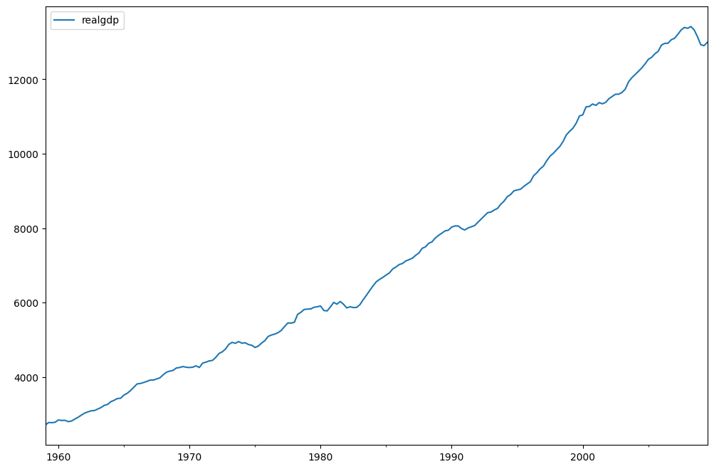
fig = plt.figure(figsize=(12, 8))
ax = fig.add_subplot(111)
dta.realgdp.plot(ax=ax)
legend = ax.legend(loc="upper left")
legend.prop.set_size(20)
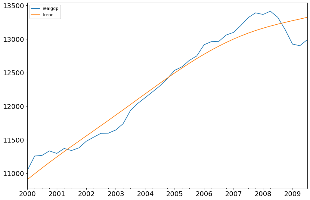
ホドリック-プレスコットフィルター
ホドリック-プレスコットフィルターは、時系列\(y_t\)をトレンド\(\tau_t\)と循環成分\(\zeta_t\)に分離します。
これらの成分は、以下の二次損失関数を最小化することによって決定されます。
[9]:
gdp_cycle, gdp_trend = sm.tsa.filters.hpfilter(dta.realgdp)
[10]:
gdp_decomp = dta[["realgdp"]].copy()
gdp_decomp["cycle"] = gdp_cycle
gdp_decomp["trend"] = gdp_trend
[11]:
fig = plt.figure(figsize=(12, 8))
ax = fig.add_subplot(111)
gdp_decomp[["realgdp", "trend"]]["2000-03-31":].plot(ax=ax, fontsize=16)
legend = ax.get_legend()
legend.prop.set_size(20)
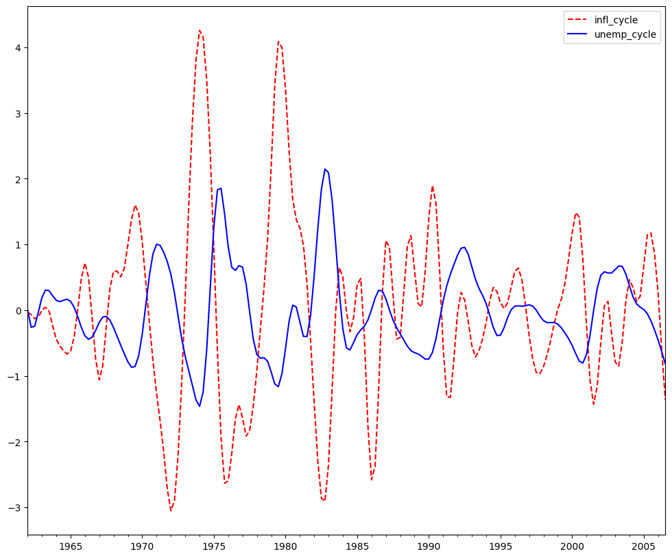
バクスター-キング近似バンドパスフィルター: インフレーションと失業
インフレーションと失業が反循環的であるという仮説を探る。
バクスター-キングフィルターは、景気循環の周期性を明示的に扱うことを目的としています。彼らのバンドパスフィルターを系列に適用することにより、景気循環の変動よりも高いまたは低い変動を含まない新しい系列を生成します。具体的には、BKフィルターは対称移動平均の形式を取ります。
ここで、\(a_{-k}=a_k\)および\(\sum_{k=-k}^{K}a_k=0\)は、系列のトレンドを削除し、系列がI(1)またはI(2)の場合に定常にするためです。
完全を期すために、フィルターの重みは次のように決定されます。
ここで、\(\theta\)は、重みの合計がゼロになるような正規化定数です。
\(P_L\)および\(P_H\)は、低および高カットオフ周波数の周期性です。米国の景気循環に関するBurns and Mitchellの研究に従い、サイクルは1.5年から8年続くとされており、デフォルトでは\(P_L=6\)および\(P_H=32\)を使用します。
[12]:
bk_cycles = sm.tsa.filters.bkfilter(dta[["infl", "unemp"]])
両端でK個の観測値を失います。四半期データにはK=12を使用することが推奨されます。
[13]:
fig = plt.figure(figsize=(12, 10))
ax = fig.add_subplot(111)
bk_cycles.plot(ax=ax, style=["r--", "b-"])
[13]:
<Axes: >
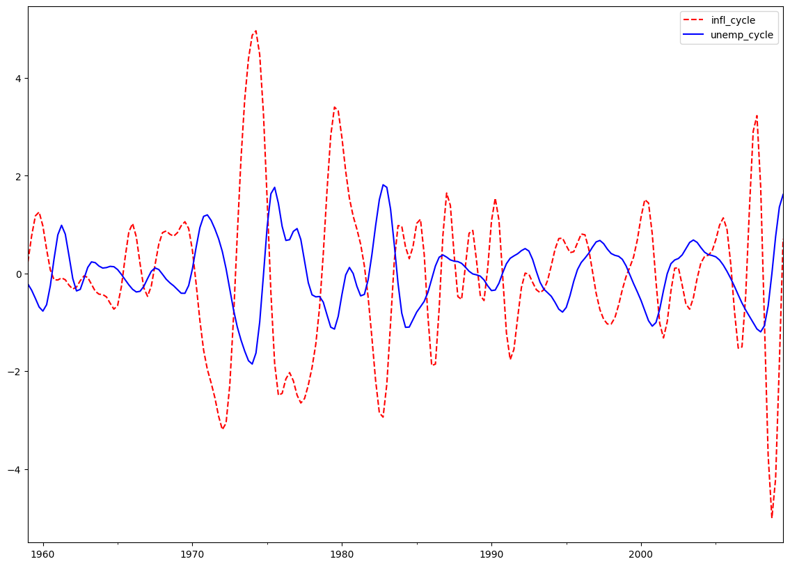
クリスティアーノ-フィッツジェラルド近似バンドパスフィルター: インフレーションと失業
クリスティアーノ-フィッツジェラルドフィルターはBKの一般化であり、したがって加重移動平均と見なすこともできます。ただし、CFフィルターは、\(t\)について非対称であるだけでなく、系列全体を使用します。彼らのフィルターの実装には、次の重みの計算が含まれます。
\(t=3,4,...,T-2\)の場合、ここで
\(\tilde B_{T-t}\)と\(\tilde B_{t-1}\)は、\(B_{j}\)の線形関数であり、\(t=1,2,T-1,\)および\(T\)の値もほぼ同じ方法で計算されます。\(P_{U}\)と\(P_{L}\)は上記の説明と同じ解釈です。
CFフィルターは、ランダムウォークに従う可能性のある系列に適しています。
[14]:
print(sm.tsa.stattools.adfuller(dta["unemp"])[:3])
(np.float64(-2.53645846733463), np.float64(0.10685366457233608), 9)
[15]:
print(sm.tsa.stattools.adfuller(dta["infl"])[:3])
(np.float64(-3.054514496257235), np.float64(0.030107620863486007), 2)
[16]:
cf_cycles, cf_trend = sm.tsa.filters.cffilter(dta[["infl", "unemp"]])
print(cf_cycles.head(10))
            infl_cycle  unemp_cycle
1959-03-31    0.237927    -0.216867
1959-06-30    0.770007    -0.343779
1959-09-30    1.177736    -0.511024
1959-12-31    1.256754    -0.686967
1960-03-31    0.972128    -0.770793
1960-06-30    0.491889    -0.640601
1960-09-30    0.070189    -0.249741
1960-12-31   -0.130432     0.301545
1961-03-31   -0.134155     0.788992
1961-06-30   -0.092073     0.985356
[17]:
fig = plt.figure(figsize=(14, 10))
ax = fig.add_subplot(111)
cf_cycles.plot(ax=ax, style=["r--", "b-"])
[17]:
<Axes: >
フィルター処理は、景気循環が存在するという事前の前提を立てます。この前提のため、多くのマクロ経済モデルは、フィルター処理された系列の特性を再現するのではなく、インパルス応答関数の形状に一致するモデルを作成しようとしています。VARノートブックを参照してください。