LOESSを用いた多重季節トレンド分解(MSTL)
このノートブックは、MSTL [1] を使用して時系列をトレンド成分、複数の季節成分、残差成分に分解する方法を示しています。MSTLは、STL(LOESSを用いた季節トレンド分解)を使用して、時系列から季節成分を反復的に抽出します。MSTLへの主要な入力は次のとおりです。
periods- 各季節成分の周期(例:日次と週次の季節性を持つ時間データの場合、periods=(24, 24*7)となります)。windows- 各周期に対する各季節スムザーの長さ。これらが大きいと、季節成分は時間とともに変動性が少なくなります。奇数でなければなりません。Noneの場合、元の論文[1]の実験で決定されたデフォルト値のセットが使用されます。lmbda- 分解前のBox-Cox変換のラムダパラメータ。Noneの場合、変換は行われません。"auto"の場合、データから適切なラムダ値が自動的に選択されます。iterate- 季節成分を洗練するために使用する反復回数。stl_kwargs- STLに渡すことができるその他すべてのパラメータ(例:robust、seasonal_degなど)。STLドキュメントを参照してください。
この実装には、1とのいくつかの重要な違いがあります。欠損データはMSTLクラスの外で処理する必要があります。論文で提案されているアルゴリズムは、季節性が存在しない場合を処理します。この実装では、少なくとも1つの季節成分があると仮定しています。
まず、必要なパッケージをインポートし、グラフィックス環境を準備し、データを準備します。
[1]:
import matplotlib.pyplot as plt
import datetime
import pandas as pd
import numpy as np
import seaborn as sns
from pandas.plotting import register_matplotlib_converters

from statsmodels.tsa.seasonal import MSTL
from statsmodels.tsa.seasonal import DecomposeResult

register_matplotlib_converters()
sns.set_style("darkgrid")
[2]:
plt.rc("figure", figsize=(16, 12))
plt.rc("font", size=13)
MSTLをトイデータセットに適用
複数の季節性を有するトイデータセットの作成
正弦波に従う日次と週次の季節性を持つ時間データを、時間単位で作成します。より現実的な例は、ノートブックの後半で示します。
[3]:
t = np.arange(1, 1000)
daily_seasonality = 5 * np.sin(2 * np.pi * t / 24)
weekly_seasonality = 10 * np.sin(2 * np.pi * t / (24 * 7))
trend = 0.0001 * t**2
y = trend + daily_seasonality + weekly_seasonality + np.random.randn(len(t))
ts = pd.date_range(start="2020-01-01", freq="H", periods=len(t))
df = pd.DataFrame(data=y, index=ts, columns=["y"])
/tmp/ipykernel_5245/288299940.py:6: FutureWarning: 'H' is deprecated and will be removed in a future version, please use 'h' instead.
  ts = pd.date_range(start="2020-01-01", freq="H", periods=len(t))
[4]:
df.head()
[4]:
| y | |
|---|---|
| 2020-01-01 00:00:00 | 2.430365 |
| 2020-01-01 01:00:00 | 1.790566 |
| 2020-01-01 02:00:00 | 4.625017 |
| 2020-01-01 03:00:00 | 7.025365 |
| 2020-01-01 04:00:00 | 7.388021 |
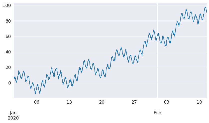
時系列をプロットしてみましょう。
[5]:
df["y"].plot(figsize=[10, 5])
[5]:
<Axes: >
MSTLによるトイデータセットの分解
MSTLを使用して、時系列をトレンド成分、日次および週次の季節成分、残差成分に分解してみましょう。
[6]:
mstl = MSTL(df["y"], periods=[24, 24 * 7])
res = mstl.fit()
入力がpandasデータフレームの場合、季節成分の出力はデータフレームになります。各成分の周期は列名に反映されます。
[7]:
res.seasonal.head()
[7]:
| seasonal_24 | seasonal_168 | |
|---|---|---|
| 2020-01-01 00:00:00 | 1.500231 | 1.796102 |
| 2020-01-01 01:00:00 | 2.339523 | 0.227047 |
| 2020-01-01 02:00:00 | 2.736665 | 2.076791 |
| 2020-01-01 03:00:00 | 5.812639 | 1.220039 |
| 2020-01-01 04:00:00 | 4.672422 | 3.259005 |
[8]:
ax = res.plot()
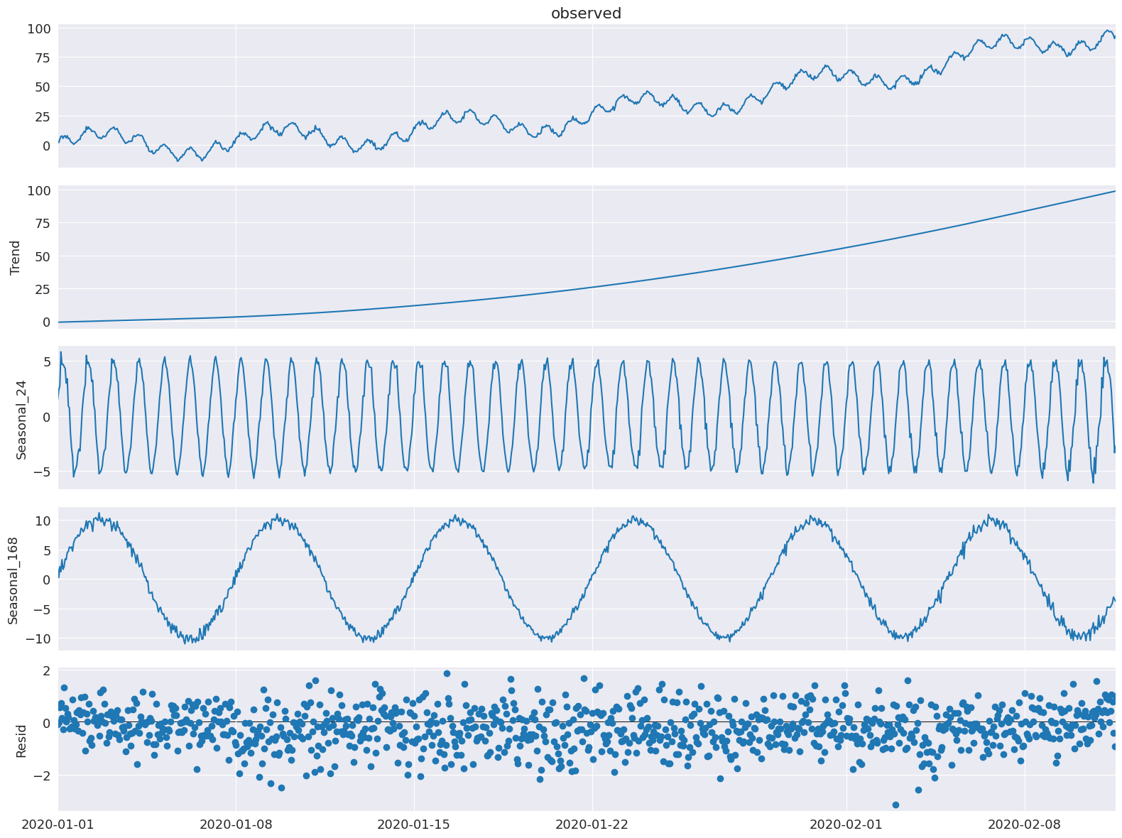
時間単位と週単位の季節成分が抽出されていることがわかります。
periodとseasonal以外のSTLパラメータ(MSTLのperiodsとwindowsで設定されるため)は、arg:valueペアを辞書としてstl_kwargsに渡すことによっても設定できます(例を以下に示します)。
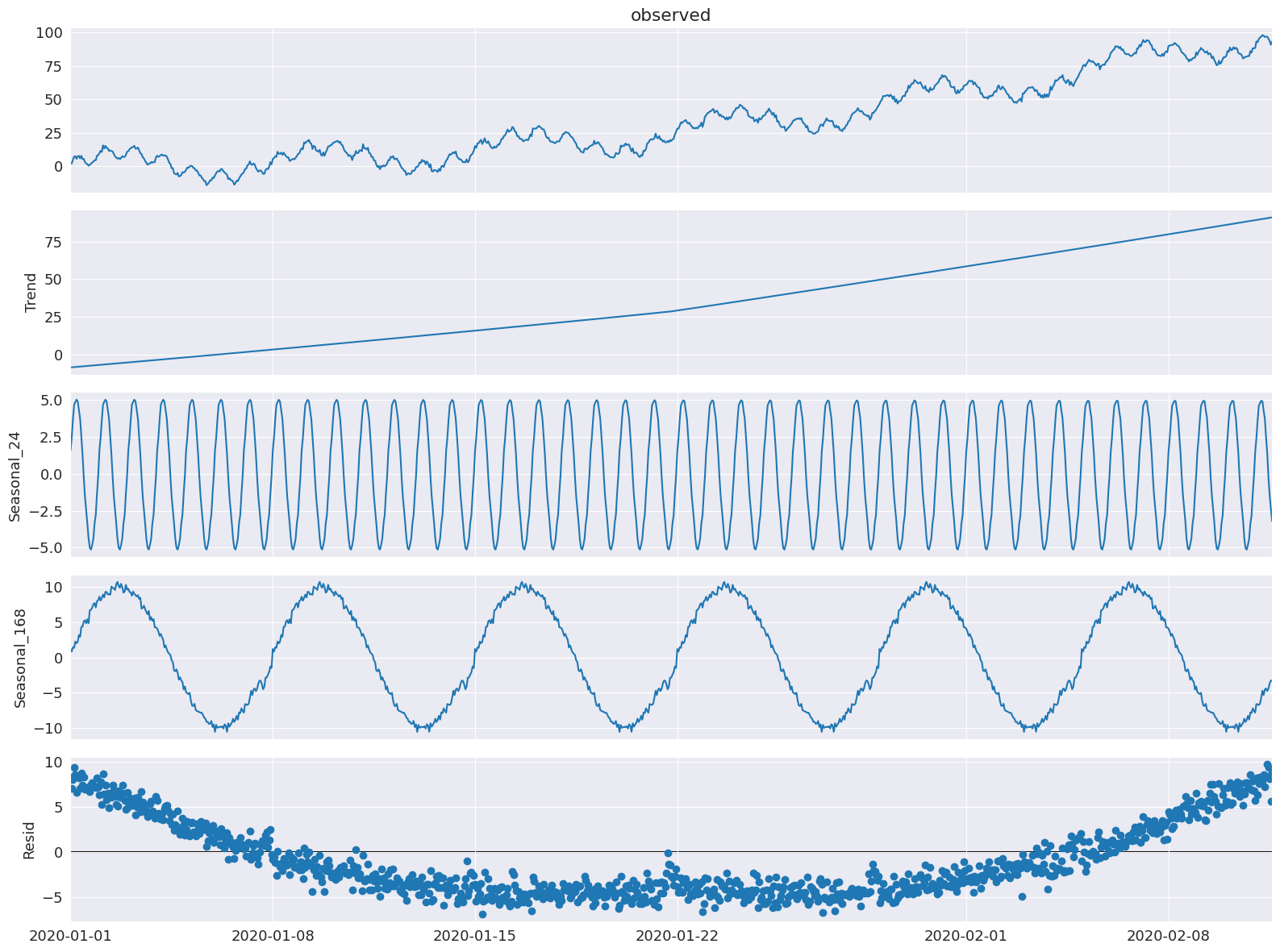
ここでは、STLのトレンドスムザーをtrendで、季節適合の多項式の次数をseasonal_degで設定できることを示します。windows、seasonal_deg、iterateパラメータも明示的に設定します。適合性は悪くなりますが、これらのパラメータをMSTLクラスに渡す方法の例です。
[9]:
mstl = MSTL(
    df,
    periods=[24, 24 * 7],  # The periods and windows must be the same length and will correspond to one another.
    windows=[101, 101],  # Setting this large along with `seasonal_deg=0` will force the seasonality to be periodic.
    iterate=3,
    stl_kwargs={
                "trend":1001, # Setting this large will force the trend to be smoother.
                "seasonal_deg":0, # Means the seasonal smoother is fit with a moving average.
               }
)
res = mstl.fit()
ax = res.plot()
MSTLを電力需要データセットに適用
データの準備
ここでは、ここに記載されているビクトリア州の電力需要データセットを使用します:https://github.com/tidyverts/tsibbledata/tree/master/data-raw/vic_elec。このデータセットは、元のMSTL論文[1]で使用されています。これは、2002年から2015年の初めまでの、オーストラリアのビクトリア州の電力需要の30分ごとのデータです。データセットの詳細な説明はこちらにあります。
[10]:
url = "https://raw.githubusercontent.com/tidyverts/tsibbledata/master/data-raw/vic_elec/VIC2015/demand.csv"
df = pd.read_csv(url)
[11]:
df.head()
[11]:
| 日付 | 期間 | OperationalLessIndustrial | Industrial | |
|---|---|---|---|---|
| 0 | 37257 | 1 | 3535.867064 | 1086.132936 |
| 1 | 37257 | 2 | 3383.499028 | 1088.500972 |
| 2 | 37257 | 3 | 3655.527552 | 1084.472448 |
| 3 | 37257 | 4 | 3510.446636 | 1085.553364 |
| 4 | 37257 | 5 | 3294.697156 | 1081.302844 |
日付は、基準日からの日数を表す整数です。このデータセットの基準日は、こちらとこちらから決定され、「1899-12-30」です。Periodの整数は、24時間の日における30分間隔を表し、したがって各日に48個あります。
日付と日時を抽出しましょう。
[12]:
df["Date"] = df["Date"].apply(lambda x: pd.Timestamp("1899-12-30") + pd.Timedelta(x, unit="days"))
df["ds"] = df["Date"] + pd.to_timedelta((df["Period"]-1)*30, unit="m")
特定の高エネルギー産業ユーザーからの需要を除いた電力需要であるOperationalLessIndustrialに関心があります。データを時間単位にリサンプリングし、元のMSTL論文[1]と同じ期間、つまり2012年の最初の149日間にデータを絞り込みます。
[13]:
timeseries = df[["ds", "OperationalLessIndustrial"]]
timeseries.columns = ["ds", "y"] # Rename to OperationalLessIndustrial to y for simplicity.

# Filter for first 149 days of 2012.
start_date = pd.to_datetime("2012-01-01")
end_date = start_date + pd.Timedelta("149D")
mask = (timeseries["ds"] >= start_date) & (timeseries["ds"] < end_date)
timeseries = timeseries[mask]

# Resample to hourly
timeseries = timeseries.set_index("ds").resample("H").sum()
timeseries.head()
/tmp/ipykernel_5245/185151541.py:11: FutureWarning: 'H' is deprecated and will be removed in a future version, please use 'h' instead.
  timeseries = timeseries.set_index("ds").resample("H").sum()
[13]:
| y | |
|---|---|
| ds | |
| 2012-01-01 00:00:00 | 7926.529376 |
| 2012-01-01 01:00:00 | 7901.826990 |
| 2012-01-01 02:00:00 | 7255.721350 |
| 2012-01-01 03:00:00 | 6792.503352 |
| 2012-01-01 04:00:00 | 6635.984460 |
MSTLを用いた電力需要の分解
このデータセットにMSTLを適用してみましょう。
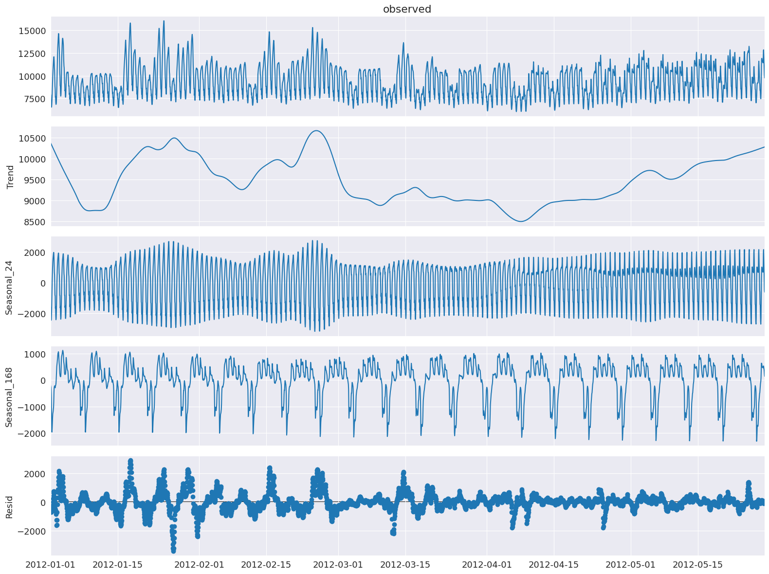
注:stl_kwargsは、Rを使用した[1]に近い結果を得るように設定されています。そのため、基礎となるSTLパラメータのデフォルト設定がわずかに異なります。inner_iterとouter_iterを明示的に設定することは、実際にはほとんどありません。
[14]:
mstl = MSTL(timeseries["y"], periods=[24, 24 * 7], iterate=3, stl_kwargs={"seasonal_deg": 0,
                                                                          "inner_iter": 2,
                                                                          "outer_iter": 0})
res = mstl.fit() # Use .fit() to perform and return the decomposition
ax = res.plot()
plt.tight_layout()
複数の季節成分は、seasonal属性にpandasデータフレームとして格納されます。
[15]:
res.seasonal.head()
[15]:
| seasonal_24 | seasonal_168 | |
|---|---|---|
| ds | ||
| 2012-01-01 00:00:00 | -1685.986297 | -161.807086 |
| 2012-01-01 01:00:00 | -1591.640845 | -229.788887 |
| 2012-01-01 02:00:00 | -2192.989492 | -260.121300 |
| 2012-01-01 03:00:00 | -2442.169359 | -388.484499 |
| 2012-01-01 04:00:00 | -2357.492551 | -660.245476 |
季節成分をもう少し詳しく調べて、最初の数日と数週間を見て、日次と週次の季節性を調べましょう。
[16]:
fig, ax = plt.subplots(nrows=2, figsize=[10,10])
res.seasonal["seasonal_24"].iloc[:24*3].plot(ax=ax[0])
ax[0].set_ylabel("seasonal_24")
ax[0].set_title("Daily seasonality")

res.seasonal["seasonal_168"].iloc[:24*7*3].plot(ax=ax[1])
ax[1].set_ylabel("seasonal_168")
ax[1].set_title("Weekly seasonality")

plt.tight_layout()
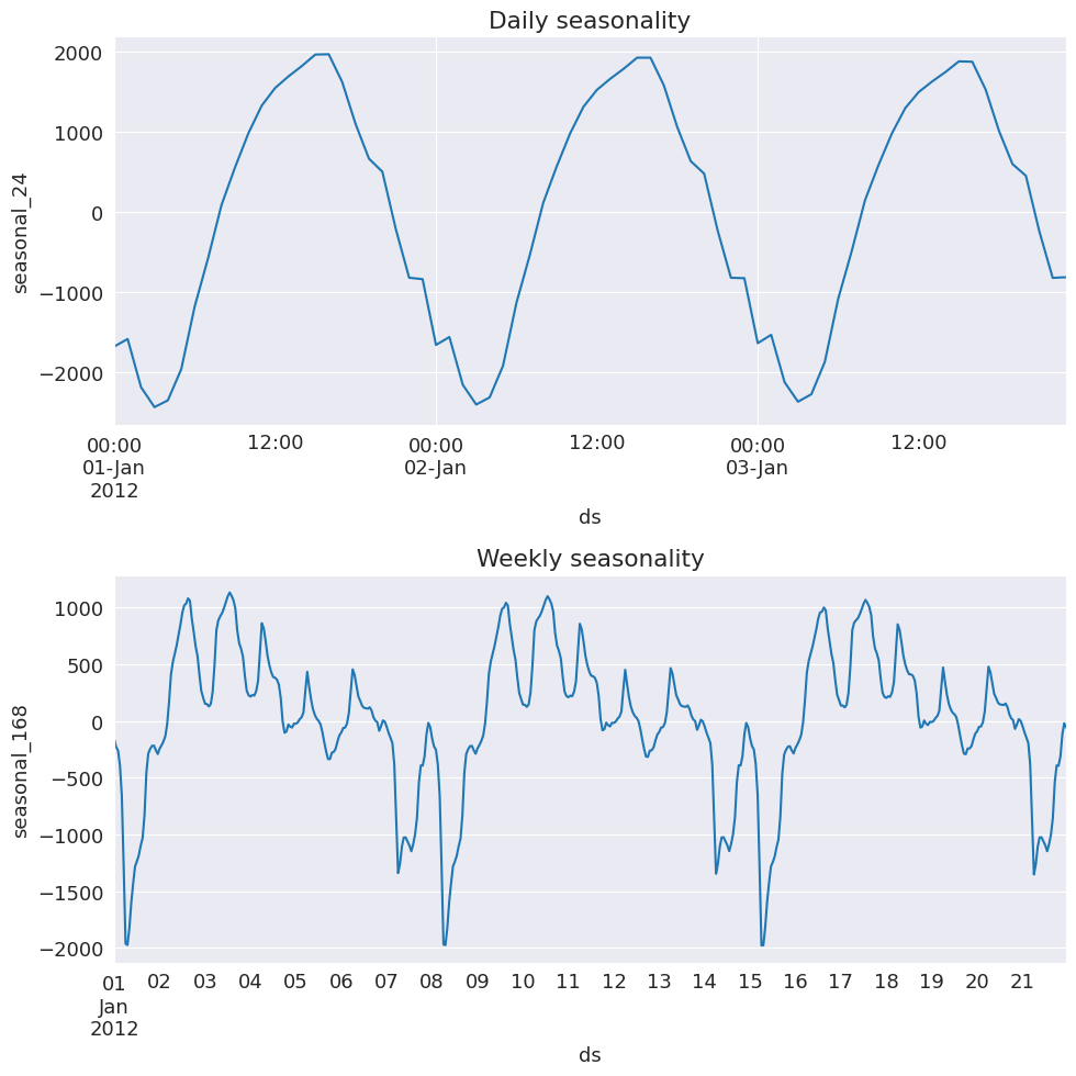
電力需要の日次季節性がうまく捉えられていることがわかります。これは1月の最初の数日なので、オーストラリアの夏の間は、おそらくエアコンの使用による午後ピークがあります。
週次の季節性については、週末は使用量が少なくなっていることがわかります。
MSTLの利点の1つは、時間とともに変化する季節性を捉えることができることです。そのため、5月の涼しい時期の季節性を調べてみましょう。
[17]:
fig, ax = plt.subplots(nrows=2, figsize=[10,10])
mask = res.seasonal.index.month==5
res.seasonal[mask]["seasonal_24"].iloc[:24*3].plot(ax=ax[0])
ax[0].set_ylabel("seasonal_24")
ax[0].set_title("Daily seasonality")

res.seasonal[mask]["seasonal_168"].iloc[:24*7*3].plot(ax=ax[1])
ax[1].set_ylabel("seasonal_168")
ax[1].set_title("Weekly seasonality")

plt.tight_layout()
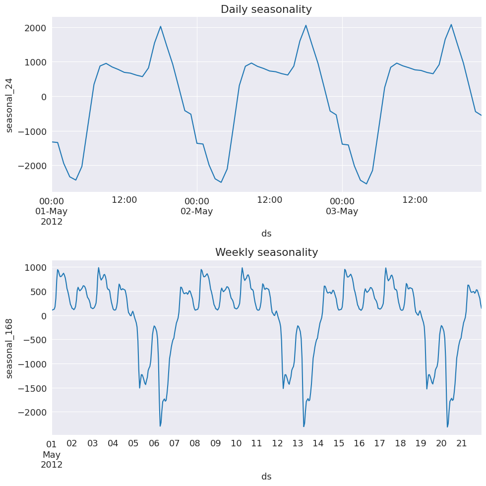
今では、夜にもピークが見られます!これは、夜間に必要となる暖房と照明に関連している可能性があります。これは理にかなっています。週末の需要が少ないという主要な週次のパターンは維持されています。
trend属性とresid属性からも他の成分を抽出できます。
[18]:
display(res.trend.head()) # trend component
display(res.resid.head()) # residual component
ds
2012-01-01 00:00:00    10373.942662
2012-01-01 01:00:00    10363.488489
2012-01-01 02:00:00    10353.037721
2012-01-01 03:00:00    10342.590527
2012-01-01 04:00:00    10332.147100
Freq: h, Name: trend, dtype: float64
ds
2012-01-01 00:00:00   -599.619903
2012-01-01 01:00:00   -640.231767
2012-01-01 02:00:00   -644.205579
2012-01-01 03:00:00   -719.433316
2012-01-01 04:00:00   -678.424613
Freq: h, Name: resid, dtype: float64
これで終わりです!MSTLを使用すると、多重季節時系列の時系列分解を実行できます!