失業におけるトレンドと循環
ここでは、経済データにおけるトレンドと循環を分離するための3つの方法を検討します。時系列データ \(y_t\) があると仮定すると、基本的な考え方は、それを以下の2つの成分に分解することです。
ここで、\(\mu_t\) はトレンドまたはレベルを表し、\(\eta_t\) は循環成分を表します。この場合、確率的トレンドを考慮するため、\(\mu_t\) はランダム変数であり、時間の決定論的関数ではありません。2つの方法は「観測されない成分」モデルの範疇に属し、3つ目は一般的なHodrick-Prescott (HP) フィルターです。たとえば、Harvey and Jaeger (1993) と一致して、これらのモデルはすべて同様の分解を生み出すことがわかりました。
このノートブックでは、これらのモデルを適用して、米国の失業率におけるトレンドと循環を分離する方法を示します。
[1]:
%matplotlib inline
[2]:
import numpy as np
import pandas as pd
import statsmodels.api as sm
import matplotlib.pyplot as plt
[3]:
from pandas_datareader.data import DataReader
endog = DataReader('UNRATE', 'fred', start='1954-01-01')
endog.index.freq = endog.index.inferred_freq
Hodrick-Prescott (HP) フィルター
最初の方法はHodrick-Prescottフィルターであり、これは非常に簡単な方法でデータ系列に適用できます。ここでは、失業率が毎月観測されるため、パラメータ \(\lambda=129600\) を指定します。
[4]:
hp_cycle, hp_trend = sm.tsa.filters.hpfilter(endog, lamb=129600)
観測されない成分とARIMAモデル (UC-ARIMA)
次の方法は、観測されない成分モデルです。ここで、トレンドはランダムウォークとしてモデル化され、循環はARIMAモデル(特にここではAR(4)モデル)でモデル化されます。時系列のプロセスは次のように書くことができます。
ここで、\(\phi(L)\) はAR(4)ラグ多項式であり、\(\epsilon_t\) と \(\nu_t\) はホワイトノイズです。
[5]:
mod_ucarima = sm.tsa.UnobservedComponents(endog, 'rwalk', autoregressive=4)
# Here the powell method is used, since it achieves a
# higher loglikelihood than the default L-BFGS method
res_ucarima = mod_ucarima.fit(method='powell', disp=False)
print(res_ucarima.summary())
                        Unobserved Components Results
==============================================================================
Dep. Variable:                 UNRATE   No. Observations:                  848
Model:                    random walk   Log Likelihood                -463.716
                              + AR(4)   AIC                            939.431
Date:                Thu, 03 Oct 2024   BIC                            967.881
Time:                        15:46:35   HQIC                           950.331
Sample:                    01-01-1954
                         - 08-01-2024
Covariance Type:                  opg
================================================================================
                   coef    std err          z      P>|z|      [0.025      0.975]
--------------------------------------------------------------------------------
sigma2.level  5.487e-08      0.011   4.92e-06      1.000      -0.022       0.022
sigma2.ar        0.1746      0.015     11.697      0.000       0.145       0.204
ar.L1            1.0256      0.019     54.095      0.000       0.988       1.063
ar.L2           -0.1059      0.016     -6.600      0.000      -0.137      -0.074
ar.L3            0.0756      0.023      3.271      0.001       0.030       0.121
ar.L4           -0.0267      0.019     -1.421      0.155      -0.064       0.010
===================================================================================
Ljung-Box (L1) (Q):                   0.00   Jarque-Bera (JB):           6657871.78
Prob(Q):                              0.97   Prob(JB):                         0.00
Heteroskedasticity (H):               9.13   Skew:                            17.46
Prob(H) (two-sided):                  0.00   Kurtosis:                       435.94
===================================================================================

Warnings:
[1] Covariance matrix calculated using the outer product of gradients (complex-step).
確率的循環を持つ観測されない成分 (UC)
最後の方法も観測されない成分モデルですが、循環が明示的にモデル化されています。
[6]:
mod_uc = sm.tsa.UnobservedComponents(
    endog, 'rwalk',
    cycle=True, stochastic_cycle=True, damped_cycle=True,
)
# Here the powell method gets close to the optimum
res_uc = mod_uc.fit(method='powell', disp=False)
# but to get to the highest loglikelihood we do a
# second round using the L-BFGS method.
res_uc = mod_uc.fit(res_uc.params, disp=False)
print(res_uc.summary())
                            Unobserved Components Results
=====================================================================================
Dep. Variable:                        UNRATE   No. Observations:                  848
Model:                           random walk   Log Likelihood                -472.478
                   + damped stochastic cycle   AIC                            952.956
Date:                       Thu, 03 Oct 2024   BIC                            971.913
Time:                               15:46:37   HQIC                           960.219
Sample:                           01-01-1954
                                - 08-01-2024
Covariance Type:                         opg
===================================================================================
                      coef    std err          z      P>|z|      [0.025      0.975]
-----------------------------------------------------------------------------------
sigma2.level        0.0183      0.033      0.552      0.581      -0.047       0.083
sigma2.cycle        0.1539      0.032      4.740      0.000       0.090       0.217
frequency.cycle     0.0437      0.029      1.495      0.135      -0.014       0.101
damping.cycle       0.9562      0.019     51.074      0.000       0.919       0.993
===================================================================================
Ljung-Box (L1) (Q):                   1.53   Jarque-Bera (JB):           6560083.72
Prob(Q):                              0.22   Prob(JB):                         0.00
Heteroskedasticity (H):               9.47   Skew:                            17.32
Prob(H) (two-sided):                  0.00   Kurtosis:                       433.26
===================================================================================

Warnings:
[1] Covariance matrix calculated using the outer product of gradients (complex-step).
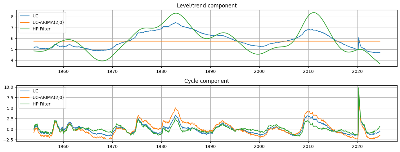
グラフによる比較
これらの各モデルの出力は、トレンド成分 \(\mu_t\) の推定値と循環成分 \(\eta_t\) の推定値です。HPフィルターのトレンド成分は、観測されない成分モデルのトレンド成分よりもいくらか変動が大きいものの、トレンドと循環の推定値は定性的に非常に似ています。これは、失業率の動きの相対的なモードは、一時的な循環的動きではなく、基礎となるトレンドの変化に起因することを意味します。
[7]:
fig, axes = plt.subplots(2, figsize=(13,5));
axes[0].set(title='Level/trend component')
axes[0].plot(endog.index, res_uc.level.smoothed, label='UC')
axes[0].plot(endog.index, res_ucarima.level.smoothed, label='UC-ARIMA(2,0)')
axes[0].plot(hp_trend, label='HP Filter')
axes[0].legend(loc='upper left')
axes[0].grid()

axes[1].set(title='Cycle component')
axes[1].plot(endog.index, res_uc.cycle.smoothed, label='UC')
axes[1].plot(endog.index, res_ucarima.autoregressive.smoothed, label='UC-ARIMA(2,0)')
axes[1].plot(hp_cycle, label='HP Filter')
axes[1].legend(loc='upper left')
axes[1].grid()

fig.tight_layout();