時系列データの季節性
周期性の異なる複数の季節成分を持つ時系列データのモデリングの問題を考えてみましょう。時系列\(y_t\)を明示的に分解して、レベル成分と2つの季節成分を持つようにします。
ここで、\(\mu_t\)はトレンドまたはレベルを表し、\(\gamma^{(1)}_t\)は比較的短い周期を持つ季節成分を表し、\(\gamma^{(2)}_t\)はより長い周期を持つ別の季節成分を表します。レベルには固定の切片項を設定し、\(\gamma^{(2)}_t\)と\(\gamma^{(2)}_t\)の両方を確率的として、季節パターンが時間とともに変化できるようにします。
このノートブックでは、このモデルに適合する合成データを生成し、観測されない成分のモデリングフレームワークの下で、いくつかの異なる方法で季節項のモデリングを実証します。
[1]:
%matplotlib inline
[2]:
import numpy as np
import pandas as pd
import statsmodels.api as sm
import matplotlib.pyplot as plt

plt.rc("figure", figsize=(16,8))
plt.rc("font", size=14)
合成データの作成
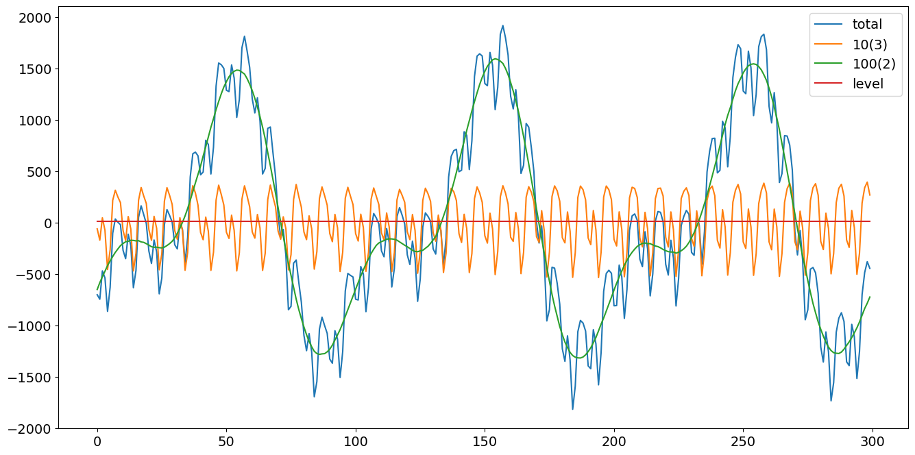
Durbin and Koopman (2012) の式(3.7)と(3.8)に従って、複数の季節パターンを持つデータを作成します。それぞれ10と100の周期と、それぞれ3と2の高調波数を持つ周波数領域でパラメータ化された、300期間と2つの季節項をシミュレートします。さらに、それらの確率的部分の分散は、それぞれ4と9です。
[3]:
# First we'll simulate the synthetic data
def simulate_seasonal_term(periodicity, total_cycles, noise_std=1.,
                           harmonics=None):
    duration = periodicity * total_cycles
    assert duration == int(duration)
    duration = int(duration)
    harmonics = harmonics if harmonics else int(np.floor(periodicity / 2))

    lambda_p = 2 * np.pi / float(periodicity)

    gamma_jt = noise_std * np.random.randn((harmonics))
    gamma_star_jt = noise_std * np.random.randn((harmonics))

    total_timesteps = 100 * duration # Pad for burn in
    series = np.zeros(total_timesteps)
    for t in range(total_timesteps):
        gamma_jtp1 = np.zeros_like(gamma_jt)
        gamma_star_jtp1 = np.zeros_like(gamma_star_jt)
        for j in range(1, harmonics + 1):
            cos_j = np.cos(lambda_p * j)
            sin_j = np.sin(lambda_p * j)
            gamma_jtp1[j - 1] = (gamma_jt[j - 1] * cos_j
                                 + gamma_star_jt[j - 1] * sin_j
                                 + noise_std * np.random.randn())
            gamma_star_jtp1[j - 1] = (- gamma_jt[j - 1] * sin_j
                                      + gamma_star_jt[j - 1] * cos_j
                                      + noise_std * np.random.randn())
        series[t] = np.sum(gamma_jtp1)
        gamma_jt = gamma_jtp1
        gamma_star_jt = gamma_star_jtp1
    wanted_series = series[-duration:] # Discard burn in

    return wanted_series
[4]:
duration = 100 * 3
periodicities = [10, 100]
num_harmonics = [3, 2]
std = np.array([2, 3])
np.random.seed(8678309)

terms = []
for ix, _ in enumerate(periodicities):
    s = simulate_seasonal_term(
        periodicities[ix],
        duration / periodicities[ix],
        harmonics=num_harmonics[ix],
        noise_std=std[ix])
    terms.append(s)
terms.append(np.ones_like(terms[0]) * 10.)
series = pd.Series(np.sum(terms, axis=0))
df = pd.DataFrame(data={'total': series,
                        '10(3)': terms[0],
                        '100(2)': terms[1],
                        'level':terms[2]})
h1, = plt.plot(df['total'])
h2, = plt.plot(df['10(3)'])
h3, = plt.plot(df['100(2)'])
h4, = plt.plot(df['level'])
plt.legend(['total','10(3)','100(2)', 'level'])
plt.show()
観測されない成分(周波数領域モデリング)
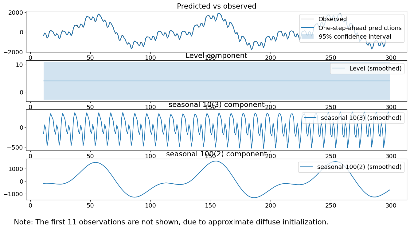
次の方法は、観測されない成分モデルです。ここでは、トレンドは固定の切片としてモデル化され、季節成分は、それぞれ10と100の主周期性を持つ三角関数を使用してモデル化され、高調波数はそれぞれ3と2です。これは正しい、生成モデルであることに注意してください。時系列のプロセスは、次のように記述できます。
ここで、\(\epsilon_t\)はホワイトノイズであり、\(\omega^{(1)}_{j,t}\)は i.i.d. \(N(0, \sigma^2_1)\)であり、\(\omega^{(2)}_{j,t}\)は i.i.d. \(N(0, \sigma^2_2)\)です。ここで、\(\sigma_1 = 2.\)です。
[5]:
model = sm.tsa.UnobservedComponents(series.values,
                                    level='fixed intercept',
                                    freq_seasonal=[{'period': 10,
                                                    'harmonics': 3},
                                                   {'period': 100,
                                                    'harmonics': 2}])
res_f = model.fit(disp=False)
print(res_f.summary())
# The first state variable holds our estimate of the intercept
print("fixed intercept estimated as {0:.3f}".format(res_f.smoother_results.smoothed_state[0,-1:][0]))

res_f.plot_components()
plt.show()
                                Unobserved Components Results
==============================================================================================
Dep. Variable:                                      y   No. Observations:                  300
Model:                                fixed intercept   Log Likelihood               -1145.631
                    + stochastic freq_seasonal(10(3))   AIC                           2295.261
                   + stochastic freq_seasonal(100(2))   BIC                           2302.594
Date:                                Thu, 03 Oct 2024   HQIC                          2298.200
Time:                                        15:59:12
Sample:                                             0
                                                - 300
Covariance Type:                                  opg
===============================================================================================
                                  coef    std err          z      P>|z|      [0.025      0.975]
-----------------------------------------------------------------------------------------------
sigma2.freq_seasonal_10(3)      4.5942      0.565      8.126      0.000       3.486       5.702
sigma2.freq_seasonal_100(2)     9.7904      2.483      3.942      0.000       4.923      14.658
===================================================================================
Ljung-Box (L1) (Q):                   0.06   Jarque-Bera (JB):                 0.08
Prob(Q):                              0.81   Prob(JB):                         0.96
Heteroskedasticity (H):               1.17   Skew:                             0.01
Prob(H) (two-sided):                  0.45   Kurtosis:                         3.08
===================================================================================

Warnings:
[1] Covariance matrix calculated using the outer product of gradients (complex-step).
fixed intercept estimated as 4.053
[6]:
model.ssm.transition[:, :, 0]
[6]:
array([[ 1.        ,  0.        ,  0.        ,  0.        ,  0.        ,
         0.        ,  0.        ,  0.        ,  0.        ,  0.        ,
         0.        ],
       [ 0.        ,  0.80901699,  0.58778525,  0.        ,  0.        ,
         0.        ,  0.        ,  0.        ,  0.        ,  0.        ,
         0.        ],
       [ 0.        , -0.58778525,  0.80901699,  0.        ,  0.        ,
         0.        ,  0.        ,  0.        ,  0.        ,  0.        ,
         0.        ],
       [ 0.        ,  0.        ,  0.        ,  0.30901699,  0.95105652,
         0.        ,  0.        ,  0.        ,  0.        ,  0.        ,
         0.        ],
       [ 0.        ,  0.        ,  0.        , -0.95105652,  0.30901699,
         0.        ,  0.        ,  0.        ,  0.        ,  0.        ,
         0.        ],
       [ 0.        ,  0.        ,  0.        ,  0.        ,  0.        ,
        -0.30901699,  0.95105652,  0.        ,  0.        ,  0.        ,
         0.        ],
       [ 0.        ,  0.        ,  0.        ,  0.        ,  0.        ,
        -0.95105652, -0.30901699,  0.        ,  0.        ,  0.        ,
         0.        ],
       [ 0.        ,  0.        ,  0.        ,  0.        ,  0.        ,
         0.        ,  0.        ,  0.99802673,  0.06279052,  0.        ,
         0.        ],
       [ 0.        ,  0.        ,  0.        ,  0.        ,  0.        ,
         0.        ,  0.        , -0.06279052,  0.99802673,  0.        ,
         0.        ],
       [ 0.        ,  0.        ,  0.        ,  0.        ,  0.        ,
         0.        ,  0.        ,  0.        ,  0.        ,  0.9921147 ,
         0.12533323],
       [ 0.        ,  0.        ,  0.        ,  0.        ,  0.        ,
         0.        ,  0.        ,  0.        ,  0.        , -0.12533323,
         0.9921147 ]])
適合された分散は、真の分散である4と9にかなり近いことに注目してください。さらに、個々の季節成分は、真の季節成分にかなり近いように見えます。平滑化されたレベル項は、真のレベルである10に近い値です。最後に、診断結果はしっかりしているように見えます。検定統計量は、3つの検定を棄却できない程度に十分に小さいです。
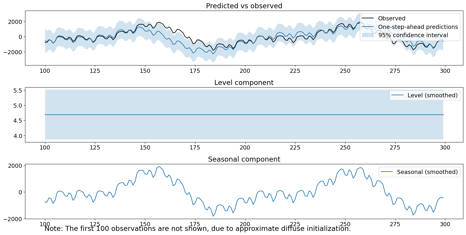
観測されない成分(混合時間・周波数領域モデリング)
2番目の方法は、観測されない成分モデルです。ここでは、トレンドは固定の切片としてモデル化され、季節成分は、合計が0になる10個の定数と、合計で2つの高調波を持つ100の主周期性を持つ三角関数を使用してモデル化されます。これは、より短い季節成分に対する状態誤差が実際よりも多いことを前提としているため、生成モデルではないことに注意してください。時系列のプロセスは、次のように記述できます。
ここで、\(\epsilon_t\)はホワイトノイズであり、\(\omega^{(1)}_{t}\)は i.i.d. \(N(0, \sigma^2_1)\)であり、\(\omega^{(2)}_{j,t}\)は i.i.d. \(N(0, \sigma^2_2)\)です。
[7]:
model = sm.tsa.UnobservedComponents(series,
                                    level='fixed intercept',
                                    seasonal=10,
                                    freq_seasonal=[{'period': 100,
                                                    'harmonics': 2}])
res_tf = model.fit(disp=False)
print(res_tf.summary())
# The first state variable holds our estimate of the intercept
print("fixed intercept estimated as {0:.3f}".format(res_tf.smoother_results.smoothed_state[0,-1:][0]))

fig = res_tf.plot_components()
fig.tight_layout(pad=1.0)
                                Unobserved Components Results
==============================================================================================
Dep. Variable:                                      y   No. Observations:                  300
Model:                                fixed intercept   Log Likelihood               -1238.113
                            + stochastic seasonal(10)   AIC                           2480.226
                   + stochastic freq_seasonal(100(2))   BIC                           2487.538
Date:                                Thu, 03 Oct 2024   HQIC                          2483.157
Time:                                        15:59:14
Sample:                                             0
                                                - 300
Covariance Type:                                  opg
===============================================================================================
                                  coef    std err          z      P>|z|      [0.025      0.975]
-----------------------------------------------------------------------------------------------
sigma2.seasonal                55.2934      7.114      7.773      0.000      41.351      69.236
sigma2.freq_seasonal_100(2)    28.6897      4.008      7.159      0.000      20.835      36.544
===================================================================================
Ljung-Box (L1) (Q):                  26.35   Jarque-Bera (JB):                 1.20
Prob(Q):                              0.00   Prob(JB):                         0.55
Heteroskedasticity (H):               1.27   Skew:                            -0.14
Prob(H) (two-sided):                  0.24   Kurtosis:                         2.87
===================================================================================

Warnings:
[1] Covariance matrix calculated using the outer product of gradients (complex-step).
fixed intercept estimated as 4.468
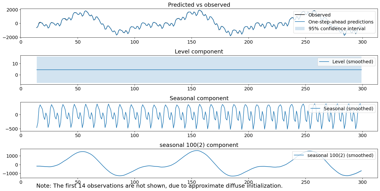
プロットされた成分はうまく見えます。ただし、2番目の季節項の推定分散は、実際よりも膨らんでいます。さらに、リュング・ボックス統計量を棄却します。これは、成分を考慮した後でも自己相関が残っている可能性があることを示しています。
観測されない成分(簡易周波数領域モデリング)
3番目の方法は、固定切片と1つの季節成分を持つ観測されない成分モデルです。この成分は、100の主周期性と50の高調波を持つ三角関数を使用してモデル化されます。これは、実際よりも多くの高調波があることを前提としているため、生成モデルではないことに注意してください。分散は結び付けられているため、存在しない高調波の推定共分散を0にすることができません。このモデル仕様の何が簡易かというと、2つの異なる季節成分をわざわざ指定せず、代わりに両方をカバーするのに十分な高調波を持つ単一の成分を使用してモデル化することを選択したことです。2つの真の成分間の分散の違いを捉えることはできません。時系列のプロセスは、次のように記述できます。
ここで、\(\epsilon_t\)はホワイトノイズであり、\(\omega^{(1)}_{t}\)は i.i.d. \(N(0, \sigma^2_1)\)です。
[8]:
model = sm.tsa.UnobservedComponents(series,
                                    level='fixed intercept',
                                    freq_seasonal=[{'period': 100}])
res_lf = model.fit(disp=False)
print(res_lf.summary())
# The first state variable holds our estimate of the intercept
print("fixed intercept estimated as {0:.3f}".format(res_lf.smoother_results.smoothed_state[0,-1:][0]))

fig = res_lf.plot_components()
fig.tight_layout(pad=1.0)
                                 Unobserved Components Results
===============================================================================================
Dep. Variable:                                       y   No. Observations:                  300
Model:                                 fixed intercept   Log Likelihood               -1101.455
                   + stochastic freq_seasonal(100(50))   AIC                           2204.910
Date:                                 Thu, 03 Oct 2024   BIC                           2208.204
Time:                                         16:06:42   HQIC                          2206.243
Sample:                                              0
                                                 - 300
Covariance Type:                                   opg
================================================================================================
                                   coef    std err          z      P>|z|      [0.025      0.975]
------------------------------------------------------------------------------------------------
sigma2.freq_seasonal_100(50)     0.7591      0.082      9.233      0.000       0.598       0.920
===================================================================================
Ljung-Box (L1) (Q):                  85.96   Jarque-Bera (JB):                 0.72
Prob(Q):                              0.00   Prob(JB):                         0.70
Heteroskedasticity (H):               1.00   Skew:                            -0.01
Prob(H) (two-sided):                  0.99   Kurtosis:                         2.71
===================================================================================

Warnings:
[1] Covariance matrix calculated using the outer product of gradients (complex-step).
fixed intercept estimated as 4.426
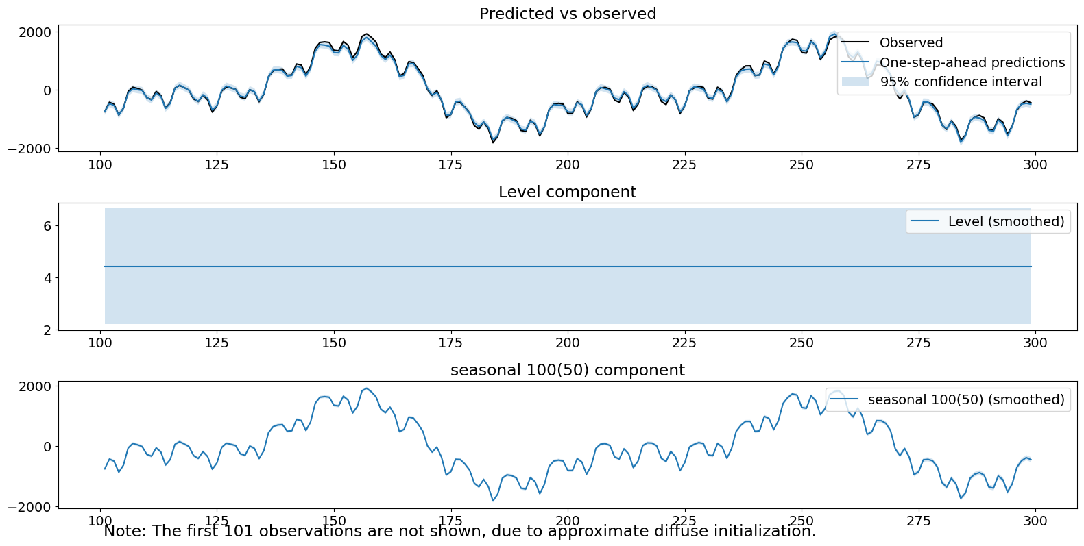
診断テストの1つは、.05レベルで棄却されることに注意してください。
観測されない成分(簡易時間領域季節性モデリング)
4番目の方法は、固定切片と100個の定数の時間領域季節モデルを使用してモデル化された単一の季節成分を持つ、観測されない成分モデルです。時系列のプロセスは、次のように記述できます。
ここで、\(\epsilon_t\)はホワイトノイズであり、\(\omega^{(1)}_{t}\)は i.i.d. \(N(0, \sigma^2_1)\)です。
[9]:
model = sm.tsa.UnobservedComponents(series,
                                    level='fixed intercept',
                                    seasonal=100)
res_lt = model.fit(disp=False)
print(res_lt.summary())
# The first state variable holds our estimate of the intercept
print("fixed intercept estimated as {0:.3f}".format(res_lt.smoother_results.smoothed_state[0,-1:][0]))

fig = res_lt.plot_components()
fig.tight_layout(pad=1.0)
                            Unobserved Components Results
======================================================================================
Dep. Variable:                              y   No. Observations:                  300
Model:                        fixed intercept   Log Likelihood               -1564.378
                   + stochastic seasonal(100)   AIC                           3130.756
Date:                        Thu, 03 Oct 2024   BIC                           3134.054
Time:                                16:07:26   HQIC                          3132.091
Sample:                                     0
                                        - 300
Covariance Type:                          opg
===================================================================================
                      coef    std err          z      P>|z|      [0.025      0.975]
-----------------------------------------------------------------------------------
sigma2.seasonal  3.558e+05   2.96e+04     12.012      0.000    2.98e+05    4.14e+05
===================================================================================
Ljung-Box (L1) (Q):                 200.79   Jarque-Bera (JB):                25.29
Prob(Q):                              0.00   Prob(JB):                         0.00
Heteroskedasticity (H):               0.49   Skew:                             0.85
Prob(H) (two-sided):                  0.00   Kurtosis:                         3.37
===================================================================================

Warnings:
[1] Covariance matrix calculated using the outer product of gradients (complex-step).
fixed intercept estimated as 4.690
季節成分自体は、主要な信号であるため、うまく見えます。季節項の推定分散は非常に高く(\(>10^5\))、ステップごとの予測に大きな不確実性が生じ、新しいデータに対する応答が遅くなります。これは、ステップごとの予測と観測における大きな誤差によって明らかになります。最後に、3つの診断テストすべてが棄却されました。
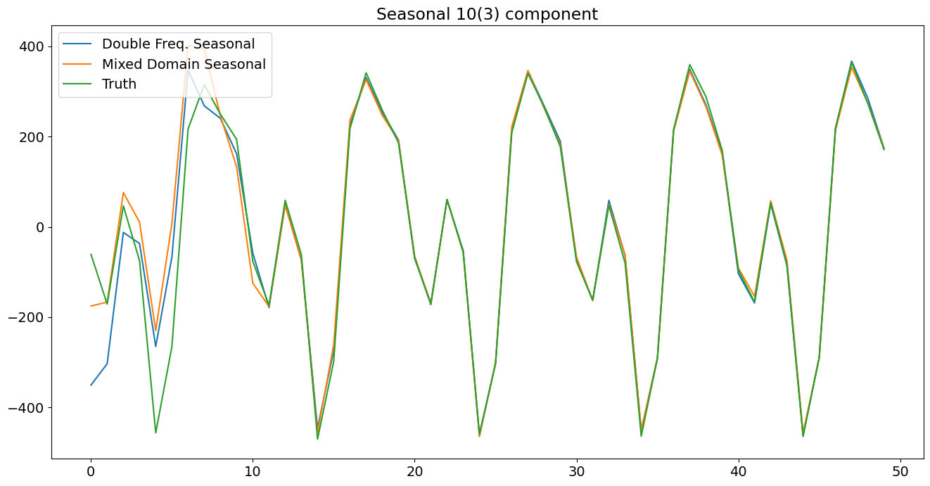
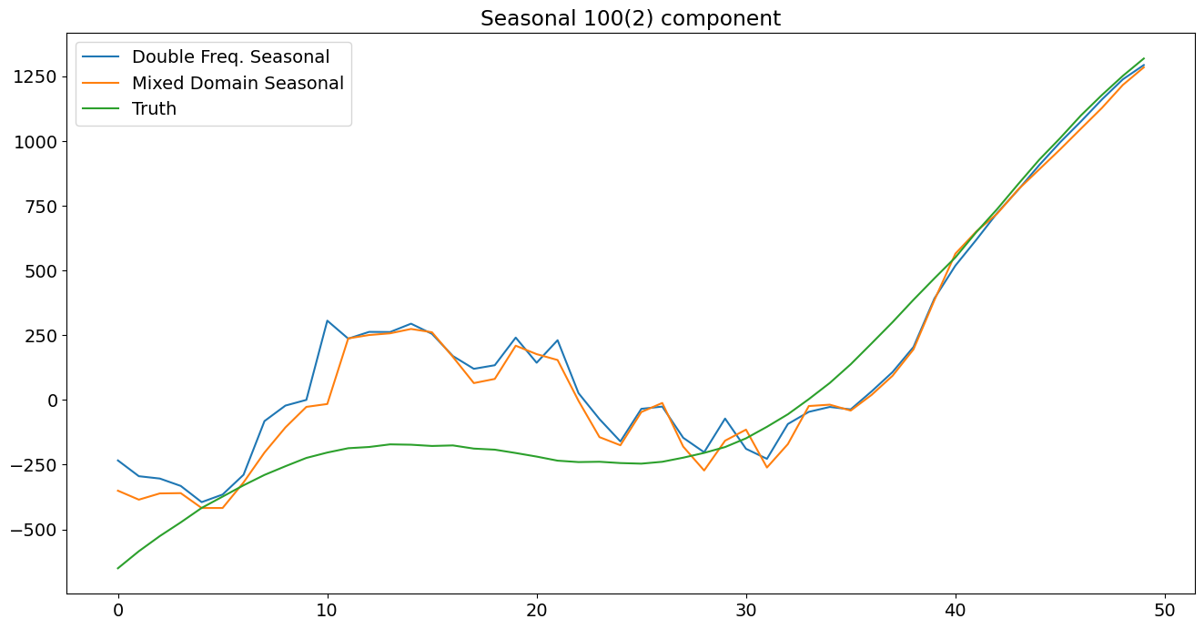
フィルター推定値の比較
以下のプロットは、個々の成分を明示的にモデル化すると、フィルター処理された状態が、およそ半周期以内に真の状態に近くなることを示しています。簡易モデルは、結合された真の状態に対して同じことを行うのに、より長い時間(ほぼ1周期)を要しました。
[10]:
# Assign better names for our seasonal terms
true_seasonal_10_3 = terms[0]
true_seasonal_100_2 = terms[1]
true_sum = true_seasonal_10_3 + true_seasonal_100_2
[11]:
time_s = np.s_[:50]  # After this they basically agree
fig1 = plt.figure()
ax1 = fig1.add_subplot(111)
idx = np.asarray(series.index)
h1, = ax1.plot(idx[time_s], res_f.freq_seasonal[0].filtered[time_s], label='Double Freq. Seas')
h2, = ax1.plot(idx[time_s], res_tf.seasonal.filtered[time_s], label='Mixed Domain Seas')
h3, = ax1.plot(idx[time_s], true_seasonal_10_3[time_s], label='True Seasonal 10(3)')
plt.legend([h1, h2, h3], ['Double Freq. Seasonal','Mixed Domain Seasonal','Truth'], loc=2)
plt.title('Seasonal 10(3) component')
plt.show()
[12]:
time_s = np.s_[:50]  # After this they basically agree
fig2 = plt.figure()
ax2 = fig2.add_subplot(111)
h21, = ax2.plot(idx[time_s], res_f.freq_seasonal[1].filtered[time_s], label='Double Freq. Seas')
h22, = ax2.plot(idx[time_s], res_tf.freq_seasonal[0].filtered[time_s], label='Mixed Domain Seas')
h23, = ax2.plot(idx[time_s], true_seasonal_100_2[time_s], label='True Seasonal 100(2)')
plt.legend([h21, h22, h23], ['Double Freq. Seasonal','Mixed Domain Seasonal','Truth'], loc=2)
plt.title('Seasonal 100(2) component')
plt.show()
[13]:
time_s = np.s_[:100]

fig3 = plt.figure()
ax3 = fig3.add_subplot(111)
h31, = ax3.plot(idx[time_s], res_f.freq_seasonal[1].filtered[time_s] + res_f.freq_seasonal[0].filtered[time_s], label='Double Freq. Seas')
h32, = ax3.plot(idx[time_s], res_tf.freq_seasonal[0].filtered[time_s] + res_tf.seasonal.filtered[time_s], label='Mixed Domain Seas')
h33, = ax3.plot(idx[time_s], true_sum[time_s], label='True Seasonal 100(2)')
h34, = ax3.plot(idx[time_s], res_lf.freq_seasonal[0].filtered[time_s], label='Lazy Freq. Seas')
h35, = ax3.plot(idx[time_s], res_lt.seasonal.filtered[time_s], label='Lazy Time Seas')

plt.legend([h31, h32, h33, h34, h35], ['Double Freq. Seasonal','Mixed Domain Seasonal','Truth', 'Lazy Freq. Seas', 'Lazy Time Seas'], loc=1)
plt.title('Seasonal components combined')
plt.tight_layout(pad=1.0)
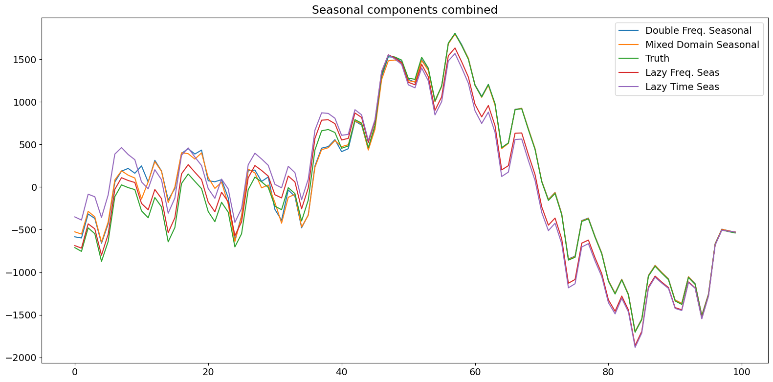
結論
このノートブックでは、異なる周期を持つ2つの季節成分を持つ時系列をシミュレーションしました。それらを構造時系列モデルを用いてモデル化しました。(a) 正しい周期と高調波の数を持つ2つの周波数領域成分、(b) 短期的な時間領域季節成分と正しい周期と高調波の数を持つ周波数領域成分、(c) 長い周期とフル高調波数を持つ単一の周波数領域成分、(d) 長い周期を持つ単一の時間領域成分です。様々な診断結果が得られましたが、正しい生成モデルである(a)のみがどのテストも棄却できませんでした。したがって、指定可能な高調波を持つ複数の成分を可能にするより柔軟な季節モデリングは、時系列モデリングに役立つツールになり得ます。最後に、季節成分をこの方法でより少ない総状態数で表現できるため、ユーザーは、多数の状態を使用し、結果として追加の分散が発生する「怠惰な」モデルを選択することを強制されるのではなく、バイアス-分散のトレードオフを自身で試みることができます。