状態空間モデルにおけるパラメータの推定または指定
このノートブックでは、statsmodelsの状態空間モデルにおいて、特定のパラメータの値を固定しつつ、他のパラメータを推定する方法を示します。
一般に、状態空間モデルでは、ユーザーは次のことが可能です。
最尤法ですべてのパラメータを推定する
いくつかのパラメータを固定し、残りを推定する
すべてのパラメータを固定する(パラメータが推定されないようにする)
[1]:
%matplotlib inline

from importlib import reload
import numpy as np
import pandas as pd
import statsmodels.api as sm
import matplotlib.pyplot as plt

from pandas_datareader.data import DataReader
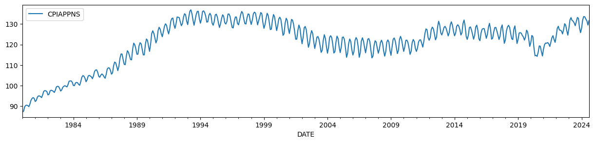
例として、時間変動するレベルと強い季節成分を持つアパレル消費者物価指数を使用します。
[2]:
endog = DataReader('CPIAPPNS', 'fred', start='1980').asfreq('MS')
endog.plot(figsize=(15, 3));
HPフィルターの出力は、パラメータに特定の制約を与えることで、観測されないコンポーネントモデルによって生成できることがよく知られています(例:Harvey and Jaeger [1993])。
観測されないコンポーネントモデルは次のとおりです。
トレンドがHPフィルターの出力と一致するためには、パラメータを次のように設定する必要があります。
ここで、\(\lambda\)は関連するHPフィルターのパラメータです。ここで使用する月次データの場合、通常\(\lambda = 129600\)が推奨されます。
[3]:
# Run the HP filter with lambda = 129600
hp_cycle, hp_trend = sm.tsa.filters.hpfilter(endog, lamb=129600)

# The unobserved components model above is the local linear trend, or "lltrend", specification
mod = sm.tsa.UnobservedComponents(endog, 'lltrend')
print(mod.param_names)
['sigma2.irregular', 'sigma2.level', 'sigma2.trend']
観測されないコンポーネントモデル(UCM)のパラメータは次のように記述されます。
\(\sigma_\varepsilon^2 = \text{sigma2.irregular}\)
\(\sigma_\eta^2 = \text{sigma2.level}\)
\(\sigma_\zeta^2 = \text{sigma2.trend}\)
上記の制約を満たすために、\((\sigma_\varepsilon^2, \sigma_\eta^2, \sigma_\zeta^2) = (1, 0, 1 / 129600)\)を設定します。
ここではすべてのパラメータを固定しているため、最尤推定を実行するために使用されるfitメソッドを使用する必要はありません。代わりに、smoothメソッドを使用して、選択したパラメータでカルマンフィルターとスムーザーを直接実行できます。
[4]:
res = mod.smooth([1., 0, 1. / 129600])
print(res.summary())
                        Unobserved Components Results
==============================================================================
Dep. Variable:               CPIAPPNS   No. Observations:                  536
Model:             local linear trend   Log Likelihood               -2997.309
Date:                Thu, 03 Oct 2024   AIC                           6000.619
Time:                        15:45:23   BIC                           6013.460
Sample:                    01-01-1980   HQIC                          6005.643
                         - 08-01-2024
Covariance Type:                  opg
====================================================================================
                       coef    std err          z      P>|z|      [0.025      0.975]
------------------------------------------------------------------------------------
sigma2.irregular     1.0000      0.009    115.621      0.000       0.983       1.017
sigma2.level              0      0.000          0      1.000      -0.000       0.000
sigma2.trend      7.716e-06   1.98e-07     38.962      0.000    7.33e-06     8.1e-06
===================================================================================
Ljung-Box (L1) (Q):                 254.28   Jarque-Bera (JB):                 1.58
Prob(Q):                              0.00   Prob(JB):                         0.45
Heteroskedasticity (H):               2.21   Skew:                             0.04
Prob(H) (two-sided):                  0.00   Kurtosis:                         2.75
===================================================================================

Warnings:
[1] Covariance matrix calculated using the outer product of gradients (complex-step).
HPフィルターのトレンド推定に対応する推定値は、levelの平滑化推定値(上記の表記では\(\mu_t\))で与えられます。
[5]:
ucm_trend = pd.Series(res.level.smoothed, index=endog.index)
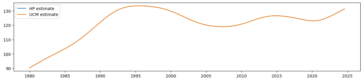
UCMからの平滑化されたレベルの推定値が、HPフィルターの出力と等しいことは容易にわかります。
[6]:
fig, ax = plt.subplots(figsize=(15, 3))

ax.plot(hp_trend, label='HP estimate')
ax.plot(ucm_trend, label='UCM estimate')
ax.legend();
季節成分の追加
ただし、観測されないコンポーネントモデルは、HPフィルターよりも柔軟性があります。たとえば、上に示したデータは明らかに季節性がありますが、季節効果は時間とともに変化します(季節性は、最初よりも最後の方がはるかに弱いです)。観測されないコンポーネントフレームワークの利点の1つは、確率的な季節成分を追加できることです。この場合、トレンドがHPフィルターの概念に対応するように、上記のパラメータに関する制約を含めながら、最尤法で季節成分の分散を推定します。
確率的な季節成分を追加すると、新しいパラメータsigma2.seasonalが1つ追加されます。
[7]:
# Construct a local linear trend model with a stochastic seasonal component of period 1 year
mod = sm.tsa.UnobservedComponents(endog, 'lltrend', seasonal=12, stochastic_seasonal=True)
print(mod.param_names)
['sigma2.irregular', 'sigma2.level', 'sigma2.trend', 'sigma2.seasonal']
この場合、上記のように最初の3つのパラメータを制限し続けますが、sigma2.seasonalの値を最尤法で推定します。したがって、fitメソッドとfix_paramsコンテキストマネージャーを使用します。
fix_paramsメソッドは、パラメータ名と関連する値の辞書を受け取ります。生成されたコンテキスト内では、これらのパラメータがすべての場合に使用されます。fitメソッドの場合、固定されていないパラメータのみが推定されます。
[8]:
# Here we restrict the first three parameters to specific values
with mod.fix_params({'sigma2.irregular': 1, 'sigma2.level': 0, 'sigma2.trend': 1. / 129600}):
    # Now we fit any remaining parameters, which in this case
    # is just `sigma2.seasonal`
    res_restricted = mod.fit()
RUNNING THE L-BFGS-B CODE

           * * *

Machine precision = 2.220D-16
 N =            1     M =           10

At X0         0 variables are exactly at the bounds

At iterate    0    f=  3.87642D+00    |proj g|=  2.27476D-01

At iterate    5    f=  3.25868D+00    |proj g|=  2.20983D-06

           * * *

Tit   = total number of iterations
Tnf   = total number of function evaluations
Tnint = total number of segments explored during Cauchy searches
Skip  = number of BFGS updates skipped
Nact  = number of active bounds at final generalized Cauchy point
Projg = norm of the final projected gradient
F     = final function value

           * * *

   N    Tit     Tnf  Tnint  Skip  Nact     Projg        F
    1      5     12      1     0     0   2.210D-06   3.259D+00
  F =   3.2586810226319427

CONVERGENCE: NORM_OF_PROJECTED_GRADIENT_<=_PGTOL
This problem is unconstrained.
あるいは、制約の辞書も受け入れるfit_constrainedメソッドを単純に使用することもできます。
[9]:
res_restricted = mod.fit_constrained({'sigma2.irregular': 1, 'sigma2.level': 0, 'sigma2.trend': 1. / 129600})
RUNNING THE L-BFGS-B CODE

           * * *

Machine precision = 2.220D-16
 N =            1     M =           10

At X0         0 variables are exactly at the bounds

At iterate    0    f=  3.87642D+00    |proj g|=  2.27476D-01

At iterate    5    f=  3.25868D+00    |proj g|=  2.20983D-06

           * * *

Tit   = total number of iterations
Tnf   = total number of function evaluations
Tnint = total number of segments explored during Cauchy searches
Skip  = number of BFGS updates skipped
Nact  = number of active bounds at final generalized Cauchy point
Projg = norm of the final projected gradient
F     = final function value

           * * *

   N    Tit     Tnf  Tnint  Skip  Nact     Projg        F
    1      5     12      1     0     0   2.210D-06   3.259D+00
  F =   3.2586810226319427

CONVERGENCE: NORM_OF_PROJECTED_GRADIENT_<=_PGTOL
This problem is unconstrained.
要約出力にはすべてのパラメータが含まれますが、最初の3つが固定されている(したがって推定されなかった)ことが示されます。
[10]:
print(res_restricted.summary())
                            Unobserved Components Results
=====================================================================================
Dep. Variable:                      CPIAPPNS   No. Observations:                  536
Model:                    local linear trend   Log Likelihood               -1746.653
                   + stochastic seasonal(12)   AIC                           3495.306
Date:                       Thu, 03 Oct 2024   BIC                           3499.566
Time:                               15:45:24   HQIC                          3496.974
Sample:                           01-01-1980
                                - 08-01-2024
Covariance Type:                         opg
============================================================================================
                               coef    std err          z      P>|z|      [0.025      0.975]
--------------------------------------------------------------------------------------------
sigma2.irregular (fixed)     1.0000        nan        nan        nan         nan         nan
sigma2.level (fixed)              0        nan        nan        nan         nan         nan
sigma2.trend (fixed)      7.716e-06        nan        nan        nan         nan         nan
sigma2.seasonal              0.0924      0.007     12.672      0.000       0.078       0.107
===================================================================================
Ljung-Box (L1) (Q):                 459.85   Jarque-Bera (JB):                38.49
Prob(Q):                              0.00   Prob(JB):                         0.00
Heteroskedasticity (H):               2.44   Skew:                             0.30
Prob(H) (two-sided):                  0.00   Kurtosis:                         4.19
===================================================================================

Warnings:
[1] Covariance matrix calculated using the outer product of gradients (complex-step).
比較のために、制約のない最尤推定(MLE)を構築します。この場合、レベルの推定値はもはやHPフィルターの概念に対応しません。
[11]:
res_unrestricted = mod.fit()
RUNNING THE L-BFGS-B CODE

           * * *

Machine precision = 2.220D-16
 N =            4     M =           10

At X0         0 variables are exactly at the bounds

At iterate    0    f=  3.63596D+00    |proj g|=  1.07339D-01
This problem is unconstrained.
At iterate    5    f=  2.03169D+00    |proj g|=  4.05225D-01
  ys=-5.696E-01  -gs= 2.818E-01 BFGS update SKIPPED

At iterate   10    f=  1.59907D+00    |proj g|=  7.62230D-01

At iterate   15    f=  1.44540D+00    |proj g|=  2.77893D-01

At iterate   20    f=  1.39111D+00    |proj g|=  1.56723D-01

At iterate   25    f=  1.38688D+00    |proj g|=  1.41002D-03

           * * *

Tit   = total number of iterations
Tnf   = total number of function evaluations
Tnint = total number of segments explored during Cauchy searches
Skip  = number of BFGS updates skipped
Nact  = number of active bounds at final generalized Cauchy point
Projg = norm of the final projected gradient
F     = final function value

           * * *

   N    Tit     Tnf  Tnint  Skip  Nact     Projg        F
    4     28     58      1     1     0   2.548D-06   1.387D+00
  F =   1.3868826049230436

CONVERGENCE: NORM_OF_PROJECTED_GRADIENT_<=_PGTOL
最後に、トレンドおよび季節成分の平滑化された推定値を取得できます。
[12]:
# Construct the smoothed level estimates
unrestricted_trend = pd.Series(res_unrestricted.level.smoothed, index=endog.index)
restricted_trend = pd.Series(res_restricted.level.smoothed, index=endog.index)

# Construct the smoothed estimates of the seasonal pattern
unrestricted_seasonal = pd.Series(res_unrestricted.seasonal.smoothed, index=endog.index)
restricted_seasonal = pd.Series(res_restricted.seasonal.smoothed, index=endog.index)
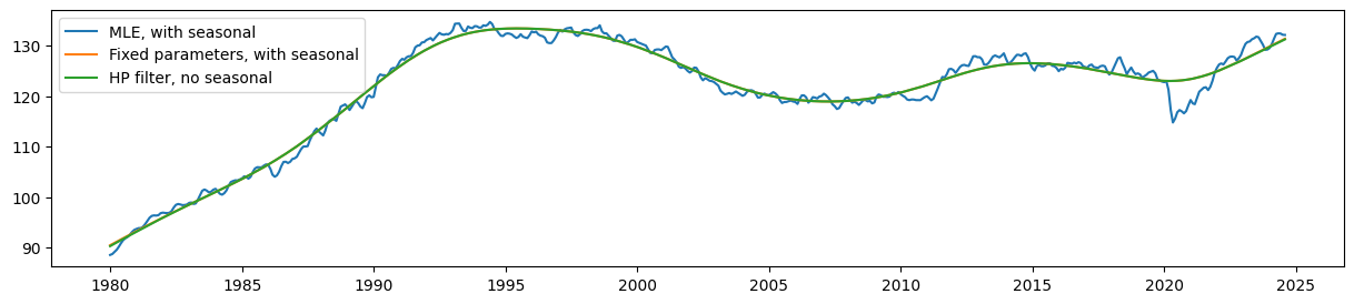
推定されたレベルを比較すると、固定パラメータを持つ季節性UCMが、HPフィルター出力に非常に近い(ただし、もはや正確ではない)トレンドを生成していることが明らかです。
一方、パラメータ制約のないモデル(MLEモデル)から推定されたレベルは、これらよりもはるかに滑らかではありません。
[13]:
fig, ax = plt.subplots(figsize=(15, 3))

ax.plot(unrestricted_trend, label='MLE, with seasonal')
ax.plot(restricted_trend, label='Fixed parameters, with seasonal')
ax.plot(hp_trend, label='HP filter, no seasonal')
ax.legend();
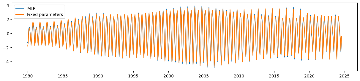
最後に、パラメータ制約のあるUCMは、時間とともに変化する季節成分を非常にうまく拾い上げることができます。
[14]:
fig, ax = plt.subplots(figsize=(15, 3))

ax.plot(unrestricted_seasonal, label='MLE')
ax.plot(restricted_seasonal, label='Fixed parameters')
ax.legend();